Chapter 36 single trial QC
What is the purpose of this notebook?
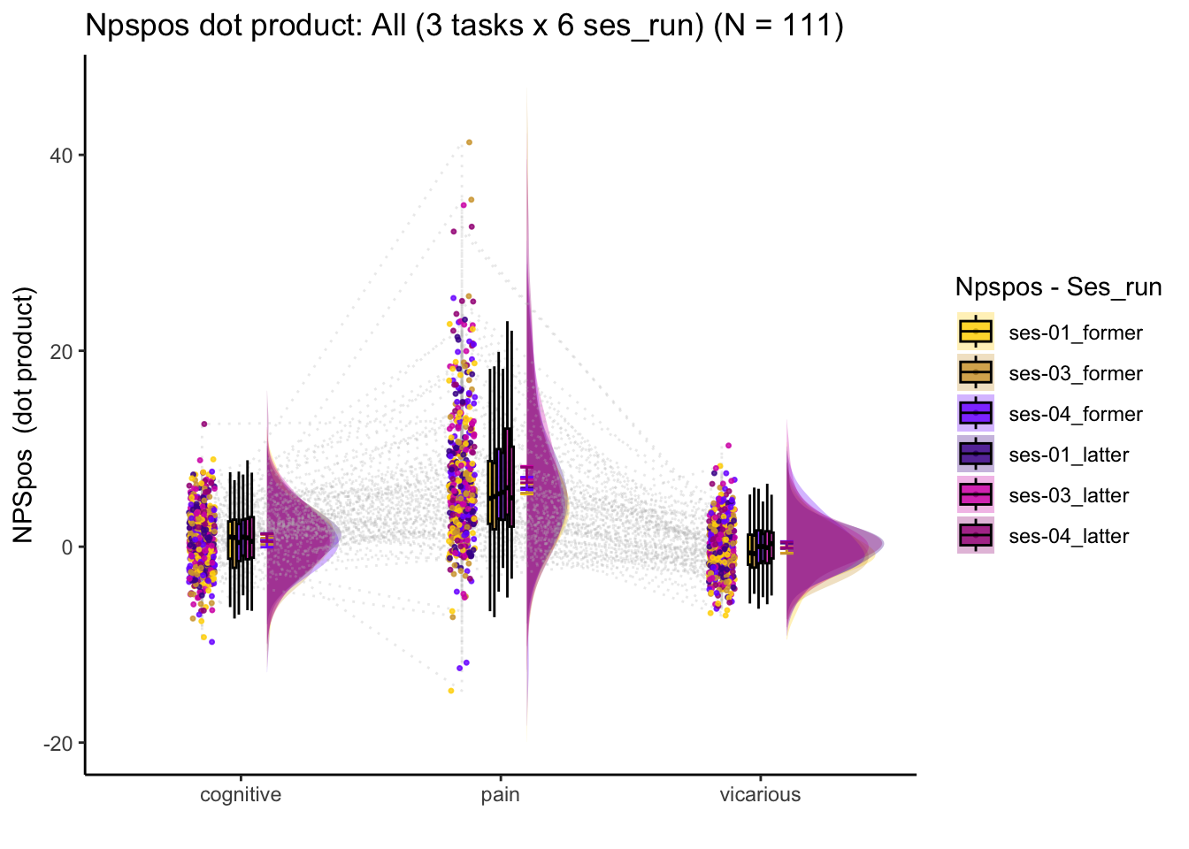
- The single trials and the univariate maps seems different, in the sense that the NPS extracted values are non-significant for the dummy univariate maps; the single trials are significant.
- Here, I test whether the order of single trials and session order has signficantly different values for NPS
Reference
https://aosmith.rbind.io/2019/04/15/custom-contrasts-emmeans/ https://aosmith.rbind.io/2019/04/15/custom-contrasts-emmeans/#:~:text=Building%20a%20custom%20contrast%20involves,0%20to%20the%20other%20groups.
trial-order wise
The purpose is to check whether trial orders have a systematic differences in average BOLD intensity, or more specifically, average NPS responses. As we can see, the first trials always have higher NPS responses. TODO: run a stats test to see if there a significant difference
36.1.1 linear model:
Q. Is this trial effect only prominent in the pain task? Q. Is this trial effect only present for the first trial of the run?
pvc$trial_num <- as.numeric(as.factor(pvc$trial))
model <-  lmer(NPSpos ~ task * trial_num + (1|sub), data = pvc)
Anova(model, type = "III")
## Analysis of Deviance Table (Type III Wald chisquare tests)
##
## Response: NPSpos
## Chisq Df Pr(>Chisq)
## (Intercept) 15.2078 1 9.630e-05 ***
## task 844.3786 2 < 2.2e-16 ***
## trial_num 2.3815 1 0.1228
## task:trial_num 22.5566 2 1.264e-05 ***
## ---
## Signif. codes: 0 '***' 0.001 '**' 0.01 '*' 0.05 '.' 0.1 ' ' 1pain = pvc[pvc$runtype == 'runtype-pain',]
pain$trialorder = as.numeric(factor(pain$trial))
# helmert_contrasts
pain$trialorder_levels <- factor(pain$trialorder,
levels=c(1,2,3,4,5,6,7,8,9,10,11,12))
pain$trial_con = factor(pain$trialorder_levels)
# contrasts(pain$trial_con) <- contrast_list
model = lmer(NPSpos ~ trial_con + (trial_con|sub), data = pain) #, contrasts = (trial_con = contrast_list))## boundary (singular) fit: see help('isSingular')## Warning: Model failed to converge with 7 negative eigenvalues: -3.9e-02 -1.4e-01
## -9.2e+00 -2.8e+01 -1.5e+02 -2.3e+02 -7.4e+02summary(model)## Linear mixed model fit by REML. t-tests use Satterthwaite's method [
## lmerModLmerTest]
## Formula: NPSpos ~ trial_con + (trial_con | sub)
## Data: pain
##
## REML criterion at convergence: 43511.1
##
## Scaled residuals:
## Min 1Q Median 3Q Max
## -5.8255 -0.4983 -0.0031 0.5013 7.0855
##
## Random effects:
## Groups Name Variance Std.Dev. Corr
## sub (Intercept) 17.2024 4.1476
## trial_con2 0.2281 0.4776 1.00
## trial_con3 2.1404 1.4630 0.84 0.84
## trial_con4 3.5478 1.8836 0.76 0.76 0.99
## trial_con5 2.8556 1.6898 0.50 0.50 0.54 0.53
## trial_con6 3.7493 1.9363 0.74 0.74 0.72 0.68 0.81
## trial_con7 2.8812 1.6974 0.66 0.66 0.74 0.72 0.44 0.86
## trial_con8 1.6353 1.2788 0.69 0.69 0.70 0.67 0.35 0.82 0.99
## trial_con9 5.1309 2.2652 0.39 0.39 0.61 0.63 0.67 0.86 0.87 0.80
## trial_con10 5.9116 2.4314 0.63 0.63 0.87 0.88 0.38 0.74 0.93 0.90
## trial_con11 7.5595 2.7495 0.48 0.48 0.72 0.76 0.80 0.54 0.27 0.17
## trial_con12 6.0055 2.4506 0.83 0.83 0.96 0.95 0.56 0.84 0.89 0.86
## Residual 75.2754 8.6761
##
##
##
##
##
##
##
##
##
##
## 0.82
## 0.46 0.45
## 0.76 0.94 0.61
##
## Number of obs: 6024, groups: sub, 109
##
## Fixed effects:
## Estimate Std. Error df t value Pr(>|t|)
## (Intercept) 9.7297 0.5569 115.0739 17.472 < 2e-16 ***
## trial_con2 -3.2064 0.5496 2818.6851 -5.834 6.01e-09 ***
## trial_con3 -3.1029 0.5658 573.6654 -5.484 6.24e-08 ***
## trial_con4 -2.3149 0.5778 337.9044 -4.007 7.58e-05 ***
## trial_con5 -3.3743 0.5729 387.5107 -5.890 8.38e-09 ***
## trial_con6 -2.6776 0.5795 362.0454 -4.620 5.34e-06 ***
## trial_con7 -3.3685 0.5725 423.0720 -5.884 8.17e-09 ***
## trial_con8 -2.6285 0.5619 746.5279 -4.678 3.44e-06 ***
## trial_con9 -3.5921 0.5925 130.0397 -6.063 1.36e-08 ***
## trial_con10 -2.9773 0.5977 208.3369 -4.981 1.33e-06 ***
## trial_con11 -3.1629 0.6122 146.5644 -5.167 7.66e-07 ***
## trial_con12 -3.8724 0.5972 253.3552 -6.485 4.63e-10 ***
## ---
## Signif. codes: 0 '***' 0.001 '**' 0.01 '*' 0.05 '.' 0.1 ' ' 1
##
## Correlation of Fixed Effects:
## (Intr) trl_c2 trl_c3 trl_c4 trl_c5 trl_c6 trl_c7 trl_c8 trl_c9
## trial_con2 -0.430
## trial_con3 -0.327 0.500
## trial_con4 -0.296 0.492 0.538
## trial_con5 -0.369 0.488 0.501 0.501
## trial_con6 -0.295 0.491 0.515 0.516 0.529
## trial_con7 -0.337 0.492 0.516 0.518 0.493 0.533
## trial_con8 -0.372 0.498 0.510 0.508 0.488 0.520 0.531
## trial_con9 -0.354 0.472 0.504 0.513 0.516 0.544 0.539 0.518
## trial_con10 -0.275 0.477 0.530 0.545 0.480 0.528 0.547 0.526 0.548
## trial_con11 -0.294 0.463 0.513 0.531 0.532 0.499 0.460 0.450 0.490
## trial_con12 -0.218 0.484 0.540 0.554 0.502 0.541 0.542 0.523 0.539
## trl_10 trl_11
## trial_con2
## trial_con3
## trial_con4
## trial_con5
## trial_con6
## trial_con7
## trial_con8
## trial_con9
## trial_con10
## trial_con11 0.486
## trial_con12 0.571 0.516
## optimizer (nloptwrap) convergence code: 0 (OK)
## boundary (singular) fit: see help('isSingular')36.1.2 trial order emmeans
## Note: D.f. calculations have been disabled because the number of observations exceeds 4000.
## To enable adjustments, add the argument 'pbkrtest.limit = 6024' (or larger)
## [or, globally, 'set emm_options(pbkrtest.limit = 6024)' or larger];
## but be warned that this may result in large computation time and memory use.
## contrast estimate SE df t.ratio p.value
## first trial vs others 3.11615 0.433 262 7.197 <.0001
## early 6 trials vs later 6 trials 0.33173 0.247 289 1.344 0.9002
## 2nd trial vs others -0.09928 0.429 294 -0.232 1.0000
## 3rd trial vs others 0.00471 0.416 487 0.011 1.0000
## 4th trial vs others 0.89177 0.421 420 2.116 0.3545
## 5th trial vs others -0.19151 0.437 270 -0.438 1.0000
## 6th trial vs others 0.58936 0.429 485 1.375 0.8861
## 7th trial vs others -0.12187 0.434 523 -0.281 1.0000
## 8th trial vs others 0.77264 0.455 238 1.696 0.6762
## 9th trial vs others -0.25460 0.473 223 -0.538 1.0000
## 10th trial vs others 0.54038 0.503 239 1.075 0.9783
## 11th trial vs 12th trial 6.21207 0.644 104 9.645 <.0001
## 1st trial vs 2nd trial 3.20640 0.550 2819 5.834 <.0001
## 12trial vs 2-11th trial -0.83184 0.420 531 -1.983 0.4497
##
## Degrees-of-freedom method: satterthwaite
## P value adjustment: mvt method for 14 testsDiscussion:
* 1st trial has high NPS values compared to other consecutive trials, across participants (t(262) = 7.197, p < .0001)
* The next thought was that there would be a linear trend. However, note that 2nd trial is not significantly different from the other trials, t(294) = -0.232, N.S. In other words, there is not linear detrending effect across trials.
* The last and 2nd-to-last trial (11th trial and 12th trial) are significantly different, t(104) = 9.645, p < .0001.
* However, it's not like the last trial is different from all others. 12th trial is not significantly different from the average of 2-11 trials, t(531) = -1.983, N.S.run wise
 ### linear model: run/ses wise
lmer(NPSpos ~ task*ses_run_con + (task|sub), data = pvc)pvc$ses_run_con <- as.factor(pvc$ses_run)
contrasts(pvc$ses_run_con) = contr.poly(6)
model_run <- lmer(NPSpos ~ task*ses_run_con + (task|sub), data = pvc)
Anova(model_run, type = "III")## Analysis of Deviance Table (Type III Wald chisquare tests)
##
## Response: NPSpos
## Chisq Df Pr(>Chisq)
## (Intercept) 17.8951 1 2.334e-05 ***
## task 165.9115 2 < 2.2e-16 ***
## ses_run_con 6.4109 5 0.268267
## task:ses_run_con 24.7977 10 0.005742 **
## ---
## Signif. codes: 0 '***' 0.001 '**' 0.01 '*' 0.05 '.' 0.1 ' ' 1summary(model_run)## Linear mixed model fit by REML. t-tests use Satterthwaite's method [
## lmerModLmerTest]
## Formula: NPSpos ~ task * ses_run_con + (task | sub)
## Data: pvc
##
## REML criterion at convergence: 133157.6
##
## Scaled residuals:
## Min 1Q Median 3Q Max
## -7.4195 -0.4787 0.0083 0.5021 8.7483
##
## Random effects:
## Groups Name Variance Std.Dev. Corr
## sub (Intercept) 2.394 1.547
## taskpain 30.314 5.506 -0.21
## taskvicarious 1.656 1.287 -0.62 0.05
## Residual 53.798 7.335
## Number of obs: 19428, groups: sub, 111
##
## Fixed effects:
## Estimate Std. Error df t value Pr(>|t|)
## (Intercept) 7.393e-01 1.748e-01 1.079e+02 4.230 4.91e-05
## taskpain 6.214e+00 5.460e-01 1.070e+02 11.381 < 2e-16
## taskvicarious -8.269e-01 1.788e-01 1.037e+02 -4.624 1.09e-05
## ses_run_con.L 2.936e-01 2.209e-01 1.914e+04 1.329 0.183807
## ses_run_con.Q 2.045e-01 2.194e-01 1.913e+04 0.932 0.351130
## ses_run_con.C -3.229e-01 2.230e-01 1.865e+04 -1.448 0.147743
## ses_run_con^4 7.937e-03 2.242e-01 1.822e+04 0.035 0.971757
## ses_run_con^5 2.940e-01 2.222e-01 1.896e+04 1.324 0.185684
## taskpain:ses_run_con.L 1.146e+00 3.246e-01 1.923e+04 3.532 0.000414
## taskvicarious:ses_run_con.L 2.598e-01 3.116e-01 1.904e+04 0.834 0.404407
## taskpain:ses_run_con.Q -2.301e-01 3.196e-01 1.913e+04 -0.720 0.471593
## taskvicarious:ses_run_con.Q -4.395e-01 3.104e-01 1.915e+04 -1.416 0.156828
## taskpain:ses_run_con.C 7.751e-02 3.297e-01 1.912e+04 0.235 0.814134
## taskvicarious:ses_run_con.C 2.674e-01 3.133e-01 1.820e+04 0.854 0.393297
## taskpain:ses_run_con^4 -4.715e-01 3.309e-01 1.904e+04 -1.425 0.154154
## taskvicarious:ses_run_con^4 1.397e-01 3.142e-01 1.752e+04 0.445 0.656609
## taskpain:ses_run_con^5 -7.010e-01 3.258e-01 1.919e+04 -2.152 0.031423
## taskvicarious:ses_run_con^5 -6.059e-01 3.127e-01 1.875e+04 -1.938 0.052654
##
## (Intercept) ***
## taskpain ***
## taskvicarious ***
## ses_run_con.L
## ses_run_con.Q
## ses_run_con.C
## ses_run_con^4
## ses_run_con^5
## taskpain:ses_run_con.L ***
## taskvicarious:ses_run_con.L
## taskpain:ses_run_con.Q
## taskvicarious:ses_run_con.Q
## taskpain:ses_run_con.C
## taskvicarious:ses_run_con.C
## taskpain:ses_run_con^4
## taskvicarious:ses_run_con^4
## taskpain:ses_run_con^5 *
## taskvicarious:ses_run_con^5 .
## ---
## Signif. codes: 0 '***' 0.001 '**' 0.01 '*' 0.05 '.' 0.1 ' ' 1##
## Correlation matrix not shown by default, as p = 18 > 12.
## Use print(x, correlation=TRUE) or
## vcov(x) if you need it36.1.3 emmeans run wise
# https://aosmith.rbind.io/2019/04/15/custom-contrasts-emmeans/
emm_options(pbkrtest.limit = 12000, lmerTest.limit = 12000)
emm <- emmeans(model_run,specs = ~task:ses_run_con, pbkrtest.limit = 12000)
## Note: D.f. calculations have been disabled because the number of observations exceeds 12000.
## To enable adjustments, add the argument 'pbkrtest.limit = 19428' (or larger)
## [or, globally, 'set emm_options(pbkrtest.limit = 19428)' or larger];
## but be warned that this may result in large computation time and memory use.## Note: D.f. calculations have been disabled because the number of observations exceeds 12000.
## To enable adjustments, add the argument 'lmerTest.limit = 19428' (or larger)
## [or, globally, 'set emm_options(lmerTest.limit = 19428)' or larger];
## but be warned that this may result in large computation time and memory use.painLinear = c(0,0,0,0,0,0,-0.5976143,-0.3585686, -0.1195229,0.1195229,0.3585686,0.5976143,0,0,0,0,0,0)
contrast(emm, method = list("painlinear" = painLinear),
adjust = "mvt") ## contrast estimate SE df z.ratio p.value
## painlinear -0.141 0.235 Inf -0.598 0.5495
##
## Degrees-of-freedom method: asymptotic