Chapter 15 [ beh ] outcome_demean ~ cue * stim * expectrating * n-1outcomerating
What is the purpose of this notebook?
Here, I model the outcome ratings as a function of cue, stimulus intensity, expectation ratings, N-1 outcome rating.
* As opposed to notebook 14, I demean the ratings within participants
* In other words, calculate the average within subjects and subtract ratings
* Main model: lmer(outcome_rating ~ cue * stim * expectation rating + N-1 outcomerating)
* Main question: What constitutes a reported outcome rating?
* Sub questions:
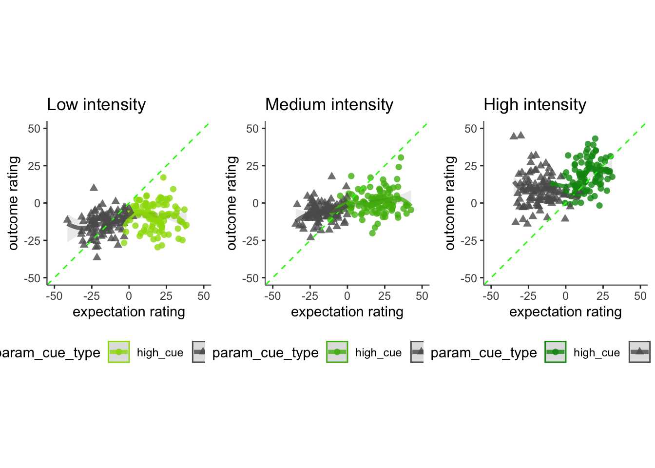
- If there is a linear relationship between expectation rating and outcome rating, does this differ as a function of cue?
- How does a N-1 outcome rating affect current expectation ratings?
- Later, is this effect different across tasks or are they similar?
- IV: stim (high / med / low) cue (high / low) expectation rating (continuous) N-1 outcome rating (continuous)
- DV: outcome rating
Some thoughts, TODOs
- Standardized coefficients
- Slope difference? Intercept difference? ( cue and expectation rating)
- Correct for the range (within participant) hypothesis:
- Larger expectation leads to prediction error
- Individual differences in ratings
- Outcome experience, based on behavioral experience What are the brain maps associated with each component.
load data and combine participant data
##  event02_expect_RT event04_actual_RT event02_expect_angle event04_actual_angle
##  Min.   :0.6504    Min.   :0.0171    Min.   :  0.00       Min.   :  0.00
##  1st Qu.:1.6200    1st Qu.:1.9188    1st Qu.: 29.55       1st Qu.: 37.83
##  Median :2.0511    Median :2.3511    Median : 57.58       Median : 60.49
##  Mean   :2.1337    Mean   :2.4011    Mean   : 61.88       Mean   : 65.47
##  3rd Qu.:2.5589    3rd Qu.:2.8514    3rd Qu.: 88.61       3rd Qu.: 87.70
##  Max.   :3.9912    Max.   :3.9930    Max.   :180.00       Max.   :180.00
## NA's :651 NA's :638 NA's :651 NA's :64115.1 linear model
## Linear mixed model fit by REML. t-tests use Satterthwaite's method [
## lmerModLmerTest]
## Formula:
## demean_outcome ~ cue_con * stim_factor * demean_expect + lag.demean_outcome +
##     (1 | src_subject_id)
##    Data: pvc
##
## REML criterion at convergence: 40138.2
##
## Scaled residuals:
##     Min      1Q  Median      3Q     Max
## -5.6623 -0.5828  0.0061  0.5953  5.5070
##
## Random effects:
##  Groups         Name        Variance Std.Dev.
##  src_subject_id (Intercept)   0.0     0.00
##  Residual                   345.2    18.58
## Number of obs: 4621, groups:  src_subject_id, 104
##
## Fixed effects:
##                                             Estimate Std. Error         df
## (Intercept)                                1.389e+01  5.931e-01  4.608e+03
## cue_con                                    9.174e-01  1.191e+00  4.608e+03
## stim_factorlow_stim                       -3.123e+01  8.560e-01  4.608e+03
## stim_factormed_stim                       -1.288e+01  8.348e-01  4.608e+03
## demean_expect                              2.573e-01  2.102e-02  4.608e+03
## lag.demean_outcome                         2.100e-01  1.148e-02  4.608e+03
## cue_con:stim_factorlow_stim               -1.292e+00  1.712e+00  4.608e+03
## cue_con:stim_factormed_stim               -5.870e+00  1.670e+00  4.608e+03
## cue_con:demean_expect                      9.867e-02  4.157e-02  4.608e+03
## stim_factorlow_stim:demean_expect         -3.067e-03  3.006e-02  4.608e+03
## stim_factormed_stim:demean_expect          1.294e-02  2.967e-02  4.608e+03
## cue_con:stim_factorlow_stim:demean_expect -2.192e-01  6.016e-02  4.608e+03
## cue_con:stim_factormed_stim:demean_expect -1.754e-01  5.936e-02  4.608e+03
##                                           t value Pr(>|t|)
## (Intercept)                                23.427  < 2e-16 ***
## cue_con                                     0.770 0.441323
## stim_factorlow_stim                       -36.480  < 2e-16 ***
## stim_factormed_stim                       -15.423  < 2e-16 ***
## demean_expect                              12.240  < 2e-16 ***
## lag.demean_outcome                         18.288  < 2e-16 ***
## cue_con:stim_factorlow_stim                -0.755 0.450499
## cue_con:stim_factormed_stim                -3.516 0.000443 ***
## cue_con:demean_expect                       2.373 0.017665 *
## stim_factorlow_stim:demean_expect          -0.102 0.918724
## stim_factormed_stim:demean_expect           0.436 0.662732
## cue_con:stim_factorlow_stim:demean_expect  -3.644 0.000271 ***
## cue_con:stim_factormed_stim:demean_expect  -2.955 0.003145 **
## ---
## Signif. codes:  0 '***' 0.001 '**' 0.01 '*' 0.05 '.' 0.1 ' ' 1
## optimizer (nloptwrap) convergence code: 0 (OK)
## boundary (singular) fit: see help('isSingular')
15.2 Q. Are those overestimating for high cues also underestimators for low cues?
y axis: oiutcome rating x axis: high cue
distance from 1:1 line
## boundary (singular) fit: see help('isSingular')## Warning: Model failed to converge with 1 negative eigenvalue: -4.1e+01## Linear mixed model fit by REML. t-tests use Satterthwaite's method [
## lmerModLmerTest]
## Formula:
## as.formula(reformulate(c(iv, sprintf("(%s|%s)", iv, subject_keyword)),
## response = dv))
## Data: df
##
## REML criterion at convergence: 39285.8
##
## Scaled residuals:
## Min 1Q Median 3Q Max
## -3.1336 -0.6750 -0.1283 0.5529 6.1548
##
## Random effects:
## Groups Name Variance Std.Dev. Corr
## src_subject_id (Intercept) 67.035 8.188
## cue_namelow 2.446 1.564 1.00
## Residual 272.378 16.504
## Number of obs: 4621, groups: src_subject_id, 104
##
## Fixed effects:
## Estimate Std. Error df t value Pr(>|t|)
## (Intercept) 23.1749 0.8848 103.1533 26.191 <2e-16 ***
## cue_namelow 0.4760 0.5104 516.1840 0.933 0.351
## ---
## Signif. codes: 0 '***' 0.001 '**' 0.01 '*' 0.05 '.' 0.1 ' ' 1
##
## Correlation of Fixed Effects:
## (Intr)
## cue_namelow 0.013
## optimizer (nloptwrap) convergence code: 0 (OK)
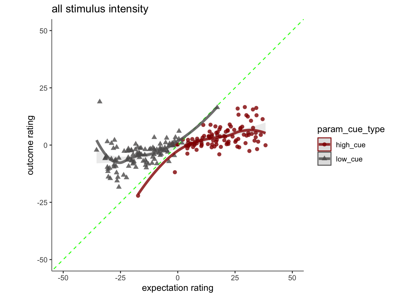
## boundary (singular) fit: see help('isSingular')Can you test if the slopes are the same? That might tell us something about whether, expectancies translate into outcomes with the same efficacy across all three tasks.
## Warning: Model failed to converge with 1 negative eigenvalue: -4.1e+01## Linear mixed model fit by REML. t-tests use Satterthwaite's method [
## lmerModLmerTest]
## Formula:
## as.formula(reformulate(c(iv, sprintf("(%s|%s)", iv, subject_keyword)),
## response = dv))
## Data: df
##
## REML criterion at convergence: 39285.8
##
## Scaled residuals:
## Min 1Q Median 3Q Max
## -3.1336 -0.6750 -0.1283 0.5529 6.1548
##
## Random effects:
## Groups Name Variance Std.Dev. Corr
## src_subject_id (Intercept) 67.035 8.188
## cue_namelow 2.446 1.564 1.00
## Residual 272.378 16.504
## Number of obs: 4621, groups: src_subject_id, 104
##
## Fixed effects:
## Estimate Std. Error df t value Pr(>|t|)
## (Intercept) 23.1749 0.8848 103.1533 26.191 <2e-16 ***
## cue_namelow 0.4760 0.5104 516.1840 0.933 0.351
## ---
## Signif. codes: 0 '***' 0.001 '**' 0.01 '*' 0.05 '.' 0.1 ' ' 1
##
## Correlation of Fixed Effects:
## (Intr)
## cue_namelow 0.013
## optimizer (nloptwrap) convergence code: 0 (OK)
## boundary (singular) fit: see help('isSingular')## Warning in geom_line(data = subjectwise, aes(group = .data[[subject]], x =
## as.numeric(as.factor(.data[[iv]])) - : Ignoring unknown aesthetics: fill## Warning: Removed 1 rows containing non-finite values (`stat_half_ydensity()`).## Warning: Removed 1 rows containing non-finite values (`stat_boxplot()`).## Warning: Removed 1 row containing missing values (`geom_line()`).## Warning: Removed 1 rows containing missing values (`geom_point()`).## Warning: Removed 1 rows containing non-finite values (`stat_half_ydensity()`).## Warning: Removed 1 rows containing non-finite values (`stat_boxplot()`).## Warning: Removed 1 row containing missing values (`geom_line()`).## Warning: Removed 1 rows containing missing values (`geom_point()`).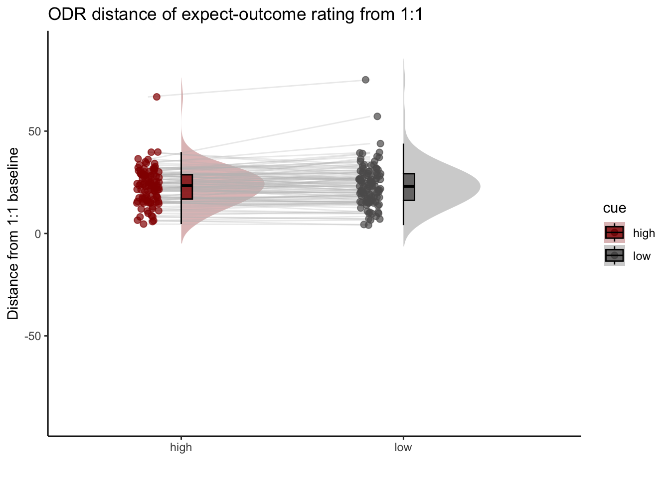
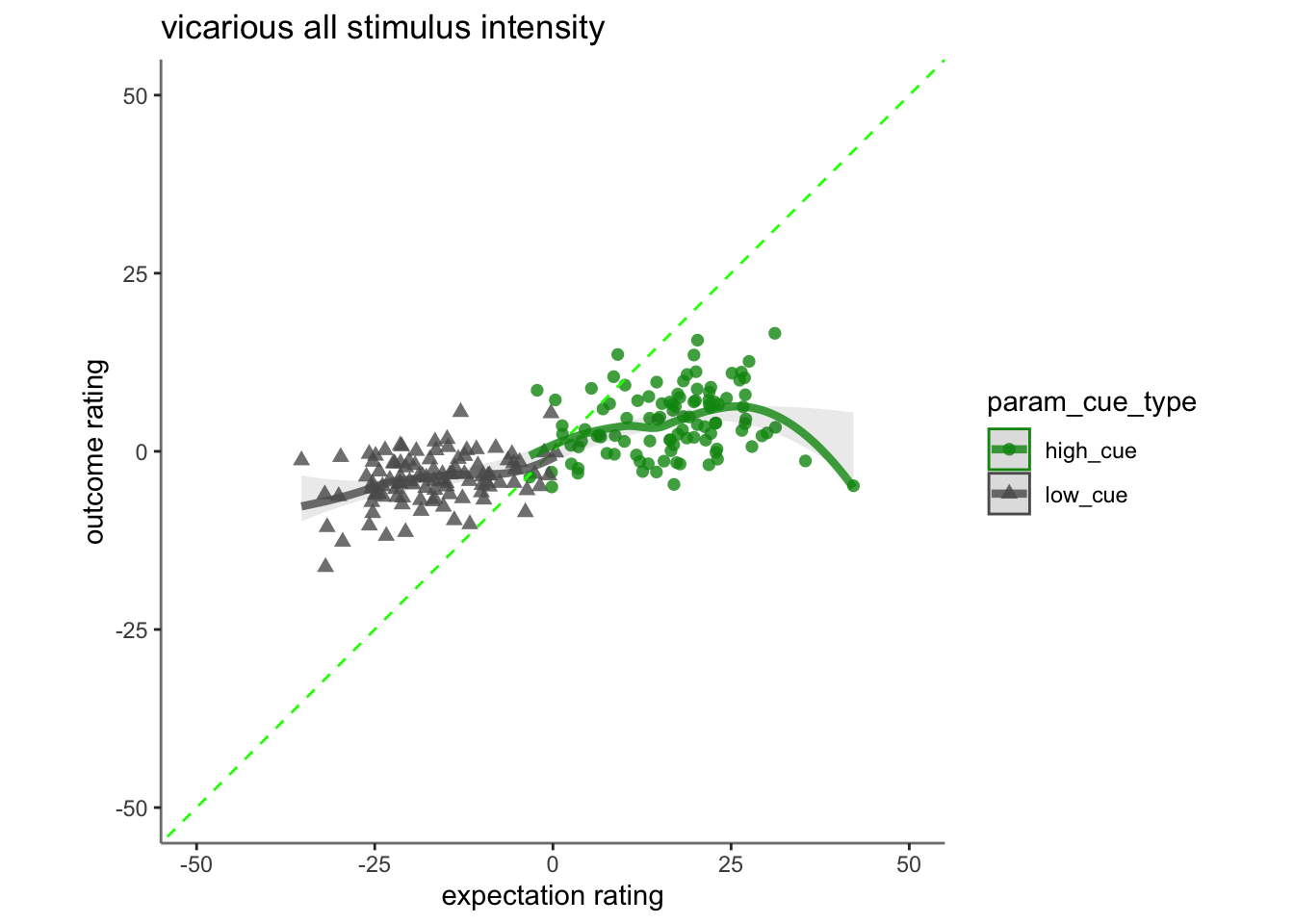
15.4 vicarious
## Linear mixed model fit by REML. t-tests use Satterthwaite's method [
## lmerModLmerTest]
## Formula:
## as.formula(reformulate(c(iv, sprintf("(%s|%s)", iv, subject_keyword)),
##     response = dv))
##    Data: df
##
## REML criterion at convergence: 40110.9
##
## Scaled residuals:
##     Min      1Q  Median      3Q     Max
## -2.8841 -0.6851 -0.1162  0.5364  5.2303
##
## Random effects:
##  Groups         Name        Variance Std.Dev. Corr
##  src_subject_id (Intercept)  47.4951  6.892
##                 cue_namelow   0.0228  0.151   -1.00
##  Residual                   236.8877 15.391
## Number of obs: 4802, groups:  src_subject_id, 104
##
## Fixed effects:
##              Estimate Std. Error        df t value Pr(>|t|)
## (Intercept)   20.5550     0.7549  105.0633  27.229   <2e-16 ***
## cue_namelow   -0.5205     0.4455 4234.0518  -1.168    0.243
## ---
## Signif. codes:  0 '***' 0.001 '**' 0.01 '*' 0.05 '.' 0.1 ' ' 1
##
## Correlation of Fixed Effects:
##             (Intr)
## cue_namelow -0.328
## optimizer (nloptwrap) convergence code: 0 (OK)
## boundary (singular) fit: see help('isSingular')
## Warning in geom_line(data = subjectwise, aes(group = .data[[subject]], x =
## as.numeric(as.factor(.data[[iv]])) - : Ignoring unknown aesthetics: fill## Warning: Removed 1 rows containing non-finite values (`stat_half_ydensity()`).## Warning: Removed 1 rows containing non-finite values (`stat_boxplot()`).## Warning: Removed 1 row containing missing values (`geom_line()`).## Warning: Removed 1 rows containing missing values (`geom_point()`).## Warning: Removed 1 rows containing non-finite values (`stat_half_ydensity()`).## Warning: Removed 1 rows containing non-finite values (`stat_boxplot()`).## Warning: Removed 1 row containing missing values (`geom_line()`).## Warning: Removed 1 rows containing missing values (`geom_point()`).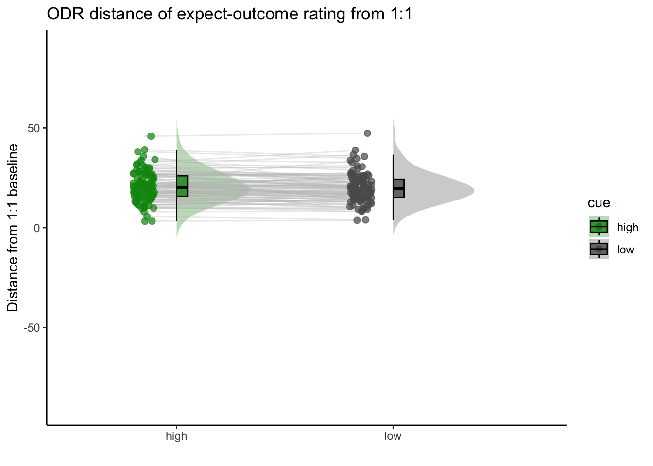
15.5 cognitive
## Linear mixed model fit by REML. t-tests use Satterthwaite's method [
## lmerModLmerTest]
## Formula:
## as.formula(reformulate(c(iv, sprintf("(%s|%s)", iv, subject_keyword)),
##     response = dv))
##    Data: df
##
## REML criterion at convergence: 38340.3
##
## Scaled residuals:
##     Min      1Q  Median      3Q     Max
## -2.4766 -0.6631 -0.1333  0.5071  6.6831
##
## Random effects:
##  Groups         Name        Variance  Std.Dev. Corr
##  src_subject_id (Intercept)  44.45232  6.6673
##                 cue_namelow   0.02064  0.1437  -1.00
##  Residual                   187.79614 13.7039
## Number of obs: 4719, groups:  src_subject_id, 104
##
## Fixed effects:
##              Estimate Std. Error        df t value Pr(>|t|)
## (Intercept)   18.9099     0.7192  101.7148  26.293   <2e-16 ***
## cue_namelow   -0.5223     0.4003 4083.1539  -1.305    0.192
## ---
## Signif. codes:  0 '***' 0.001 '**' 0.01 '*' 0.05 '.' 0.1 ' ' 1
##
## Correlation of Fixed Effects:
##             (Intr)
## cue_namelow -0.311
## optimizer (nloptwrap) convergence code: 0 (OK)
## boundary (singular) fit: see help('isSingular')
## Warning in geom_line(data = subjectwise, aes(group = .data[[subject]], x =
## as.numeric(as.factor(.data[[iv]])) - : Ignoring unknown aesthetics: fill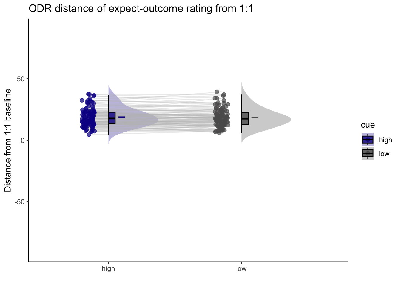
# library(plotly)
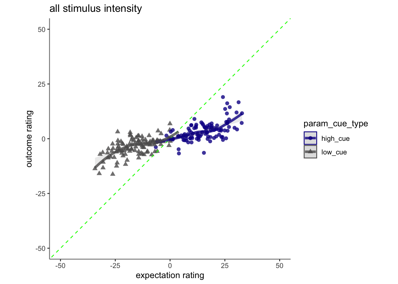
# plot_ly(x=subjectwise_naomit_2dv$param_cue_type, y=subjectwise_naomit_2dv$DV1_mean_per_sub, z=subjectwise_naomit_2dv$DV2_mean_per_sub, type="scatter3d", mode="markers", color=subjectwise_naomit_2dv$param_cue_type)15.6 across tasks (PVC), is the slope for (highvslow cue) the same?Tor question
- Adding “participant” as random effects leads to a singular boundary issue. The reason is because there is no random effects variance across participants.
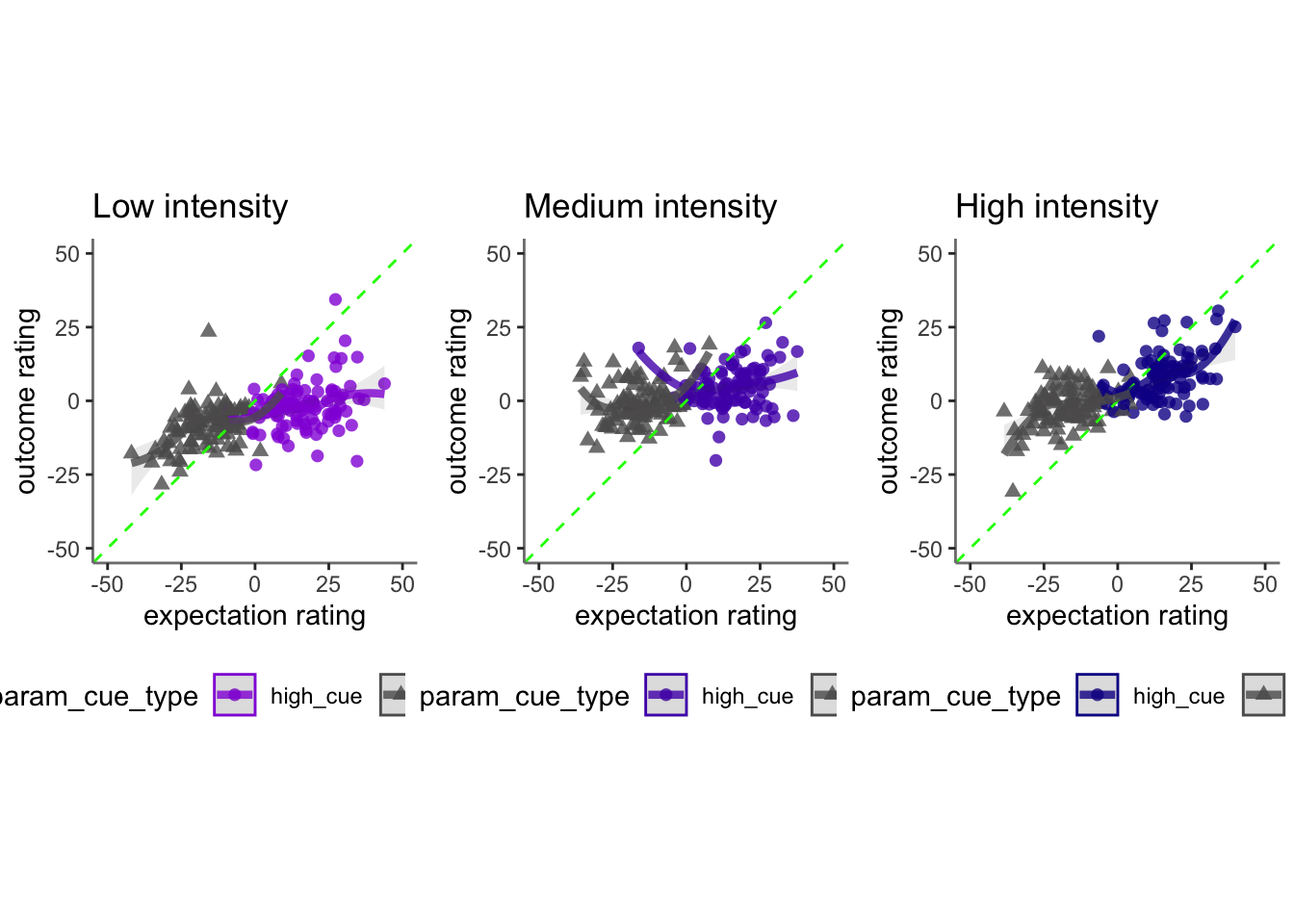
- If I add task as a random effect, in other words, allowing for differences across tasks, I get the following results:
- expectancy-outcome relationship differs across tasks, taskname_lin:demean_expect, t(14130) = 4.317, p < .001
- expectancy-outcome relationship differs across cue and tasks, “taskname_lin:cue_con:demean_expect”, t(14130) = 5.758, p < .001 taskname_lin:cue_con -3.790e+00 1.448e+00 1.413e+04 -2.618 0.00886 ** ++ taskname_lin:demean_expect 9.854e-02 2.283e-02 1.413e+04 4.317 1.59e-05 cue_con:demean_expect -9.077e-02 1.987e-02 1.413e+04 -4.569 4.95e-06 cue_con:taskname_quad 5.352e+00 1.334e+00 1.413e+04 4.012 6.04e-05 demean_expect:taskname_quad -1.596e-01 2.253e-02 1.413e+04 -7.084 1.47e-12 taskname_lin:cue_con:demean_expect 2.629e-01 4.565e-02 1.413e+04 5.758 8.67e-09 ** cue_con:demean_expect:taskname_quad -1.021e-01 4.505e-02 1.413e+04 -2.266 0.02348
- If I add sub as random effect and ignore singular. Plus, if I remove the cue contrast…
- expectancy-outcome relationship differs across tasks, factor(param_task_name):demean_expect, F(2, 14136) = 54.765, p < .001
p <- load_task_social_df(datadir, taskname = 'pain', subject_varkey = subject_varkey, iv = iv, exclude = exclude)
v <- load_task_social_df(datadir, taskname = 'vicarious', subject_varkey = subject_varkey, iv = iv, exclude = exclude)
c <- load_task_social_df(datadir, taskname = 'cognitive', subject_varkey = subject_varkey, iv = iv, exclude = exclude)
p_sub <- p[, c("param_task_name", "param_cue_type", "src_subject_id","session_id", "param_run_num", "param_stimulus_type", "event04_actual_angle", "event02_expect_angle")]
v_sub <- v[, c("param_task_name", "param_cue_type", "src_subject_id","session_id", "param_run_num", "param_stimulus_type", "event04_actual_angle", "event02_expect_angle")]
c_sub <- c[, c("param_task_name", "param_cue_type", "src_subject_id", "session_id", "param_run_num","param_stimulus_type", "event04_actual_angle", "event02_expect_angle")]
pvc_sub <- do.call("rbind", list(p_sub, v_sub, c_sub))
maindata <- pvc_sub %>%
group_by(src_subject_id) %>%
mutate(event04_actual_angle = as.numeric(event04_actual_angle)) %>%
mutate(event02_expect_angle = as.numeric(event02_expect_angle)) %>%
mutate(avg_outcome = mean(event04_actual_angle, na.rm = TRUE)) %>%
mutate(demean_outcome = event04_actual_angle - avg_outcome) %>%
mutate(avg_expect = mean(event02_expect_angle, na.rm = TRUE)) %>%
mutate(demean_expect = event02_expect_angle - avg_expect)
data_p2= maindata %>%
arrange(src_subject_id ) %>%
group_by(src_subject_id) %>%
mutate(trial_index = row_number())
data_a3 <- data_p2 %>%
group_by(src_subject_id, session_id, param_run_num) %>%
mutate(trial_index = row_number(param_run_num))
data_a3lag <-
data_a3 %>%
group_by(src_subject_id, session_id, param_run_num) %>%
mutate(lag.demean_outcome = dplyr::lag(demean_outcome, n = 1, default = NA))
data_a3lag_omit <- data_a3lag[complete.cases(data_a3lag$lag.demean_outcome),]
df <- data_a3lag_omit
pvc_sub <- simple_contrasts_beh(df)## Warning: Unknown or uninitialised column: `stim_con_linear`.## Warning: Unknown or uninitialised column: `stim_con_quad`.## Warning: Unknown or uninitialised column: `cue_con`.## Warning: Unknown or uninitialised column: `cue_name`.# contrast code 1 linear
pvc_sub$taskname_lin[pvc_sub$param_task_name == "pain"] <- 0.5## Warning: Unknown or uninitialised column: `taskname_lin`.pvc_sub$taskname_lin[pvc_sub$param_task_name == "vicarious"] <- 0
pvc_sub$taskname_lin[pvc_sub$param_task_name == "cognitive"] <- -0.5
# contrast code 2 quadratic
pvc_sub$taskname_quad[pvc_sub$param_task_name == "pain"] <- -0.33## Warning: Unknown or uninitialised column: `taskname_quad`.pvc_sub$taskname_quad[pvc_sub$param_task_name == "vicarious"] <- 0.66
pvc_sub$taskname_quad[pvc_sub$param_task_name == "cognitive"] <- -0.33
pvc_sub$sub = factor(pvc_sub$src_subject_id)
# model_test = lm(pvc_sub$demean_outcome~ pvc_sub$demean_expect)
model_task = lmer(demean_outcome~ taskname_lin*cue_con*demean_expect + taskname_quad*cue_con*demean_expect + (1 | sub), data = pvc_sub)
model_wotask = lmer(demean_outcome~ cue_con*demean_expect +(1 | sub), data = pvc_sub)## boundary (singular) fit: see help('isSingular')summary(model_task)## Linear mixed model fit by REML. t-tests use Satterthwaite's method [
## lmerModLmerTest]
## Formula:
## demean_outcome ~ taskname_lin * cue_con * demean_expect + taskname_quad *
## cue_con * demean_expect + (1 | sub)
## Data: pvc_sub
##
## REML criterion at convergence: 139399.8
##
## Scaled residuals:
## Min 1Q Median 3Q Max
## -4.5727 -0.6342 -0.1226 0.5514 5.3674
##
## Random effects:
## Groups Name Variance Std.Dev.
## sub (Intercept) 0.1232 0.351
## Residual 600.5633 24.506
## Number of obs: 15091, groups: sub, 111
##
## Fixed effects:
## Estimate Std. Error df t value
## (Intercept) -3.019e-01 2.951e-01 2.477e+02 -1.023
## taskname_lin 1.801e+01 6.935e-01 1.447e+04 25.973
## cue_con -9.551e+00 5.853e-01 1.369e+04 -16.319
## demean_expect 4.696e-01 9.457e-03 1.156e+04 49.657
## taskname_quad -1.082e+01 6.465e-01 1.482e+04 -16.741
## taskname_lin:cue_con -4.377e+00 1.388e+00 7.418e+03 -3.153
## taskname_lin:demean_expect 1.007e-01 2.163e-02 1.758e+03 4.655
## cue_con:demean_expect -8.861e-02 1.894e-02 4.064e+03 -4.679
## cue_con:taskname_quad 5.276e+00 1.294e+00 1.247e+04 4.078
## demean_expect:taskname_quad -1.730e-01 2.157e-02 8.290e+03 -8.022
## taskname_lin:cue_con:demean_expect 2.685e-01 4.314e-02 1.405e+04 6.224
## cue_con:demean_expect:taskname_quad -1.063e-01 4.310e-02 1.484e+04 -2.466
## Pr(>|t|)
## (Intercept) 0.30723
## taskname_lin < 2e-16 ***
## cue_con < 2e-16 ***
## demean_expect < 2e-16 ***
## taskname_quad < 2e-16 ***
## taskname_lin:cue_con 0.00162 **
## taskname_lin:demean_expect 3.48e-06 ***
## cue_con:demean_expect 2.98e-06 ***
## cue_con:taskname_quad 4.56e-05 ***
## demean_expect:taskname_quad 1.18e-15 ***
## taskname_lin:cue_con:demean_expect 4.98e-10 ***
## cue_con:demean_expect:taskname_quad 0.01368 *
## ---
## Signif. codes: 0 '***' 0.001 '**' 0.01 '*' 0.05 '.' 0.1 ' ' 1
##
## Correlation of Fixed Effects:
## (Intr) tsknm_l cue_cn dmn_xp tsknm_q tsknm_ln:c_ tsknm_ln:d_
## taskname_ln 0.005
## cue_con -0.188 0.369
## demean_xpct 0.224 -0.360 -0.620
## taskname_qd 0.087 -0.004 -0.299 0.280
## tsknm_ln:c_ 0.368 0.032 0.004 0.141 -0.253
## tsknm_ln:d_ -0.374 0.022 0.146 -0.281 0.256 -0.574
## c_cn:dmn_xp -0.616 0.140 0.225 -0.197 -0.142 -0.362 0.151
## c_cn:tsknm_ -0.298 -0.253 0.088 -0.143 -0.382 -0.005 -0.097
## dmn_xpct:t_ 0.271 0.240 -0.139 0.177 0.391 -0.091 0.183
## tsknm_l:_:_ 0.145 -0.572 -0.375 0.150 -0.099 0.023 -0.120
## c_cn:dmn_:_ -0.137 -0.093 0.272 -0.123 -0.659 0.239 -0.099
## c_cn:d_ c_cn:t_ dmn_:_ t_:_:_
## taskname_ln
## cue_con
## demean_xpct
## taskname_qd
## tsknm_ln:c_
## tsknm_ln:d_
## c_cn:dmn_xp
## c_cn:tsknm_ 0.281
## dmn_xpct:t_ -0.123 -0.660
## tsknm_l:_:_ -0.280 0.256 -0.099
## c_cn:dmn_:_ 0.176 0.391 -0.255 0.185anova(model_task)## Type III Analysis of Variance Table with Satterthwaite's method
## Sum Sq Mean Sq NumDF DenDF F value
## taskname_lin 405142 405142 1 14470.1 674.6035
## cue_con 159941 159941 1 13687.7 266.3187
## demean_expect 1480894 1480894 1 11560.3 2465.8423
## taskname_quad 168310 168310 1 14820.0 280.2539
## taskname_lin:cue_con 5970 5970 1 7418.2 9.9409
## taskname_lin:demean_expect 13016 13016 1 1757.8 21.6722
## cue_con:demean_expect 13146 13146 1 4063.7 21.8899
## cue_con:taskname_quad 9989 9989 1 12473.3 16.6325
## demean_expect:taskname_quad 38647 38647 1 8289.7 64.3519
## taskname_lin:cue_con:demean_expect 23266 23266 1 14053.9 38.7401
## cue_con:demean_expect:taskname_quad 3652 3652 1 14843.7 6.0802
## Pr(>F)
## taskname_lin < 2.2e-16 ***
## cue_con < 2.2e-16 ***
## demean_expect < 2.2e-16 ***
## taskname_quad < 2.2e-16 ***
## taskname_lin:cue_con 0.001623 **
## taskname_lin:demean_expect 3.477e-06 ***
## cue_con:demean_expect 2.981e-06 ***
## cue_con:taskname_quad 4.565e-05 ***
## demean_expect:taskname_quad 1.183e-15 ***
## taskname_lin:cue_con:demean_expect 4.979e-10 ***
## cue_con:demean_expect:taskname_quad 0.013681 *
## ---
## Signif. codes: 0 '***' 0.001 '**' 0.01 '*' 0.05 '.' 0.1 ' ' 1anova(model_wotask, model_task)## refitting model(s) with ML (instead of REML)## Data: pvc_sub
## Models:
## model_wotask: demean_outcome ~ cue_con * demean_expect + (1 | sub)
## model_task: demean_outcome ~ taskname_lin * cue_con * demean_expect + taskname_quad * cue_con * demean_expect + (1 | sub)
## npar AIC BIC logLik deviance Chisq Df Pr(>Chisq)
## model_wotask 6 141394 141440 -70691 141382
## model_task 14 139396 139502 -69684 139368 2014.4 8 < 2.2e-16 ***
## ---
## Signif. codes: 0 '***' 0.001 '**' 0.01 '*' 0.05 '.' 0.1 ' ' 1# summary(model_test)model_task1 = lmer(demean_outcome~ factor(param_task_name)*demean_expect + (1 | sub), data = pvc_sub)
model_wotask1 = lmer(demean_outcome~ demean_expect+ (1 | sub), data = pvc_sub)## boundary (singular) fit: see help('isSingular')summary(model_task1)## Linear mixed model fit by REML. t-tests use Satterthwaite's method [
## lmerModLmerTest]
## Formula: demean_outcome ~ factor(param_task_name) * demean_expect + (1 |
## sub)
## Data: pvc_sub
##
## REML criterion at convergence: 139725.4
##
## Scaled residuals:
## Min 1Q Median 3Q Max
## -4.2535 -0.6307 -0.1171 0.5506 5.2255
##
## Random effects:
## Groups Name Variance Std.Dev.
## sub (Intercept) 0.03748 0.1936
## Residual 613.93050 24.7776
## Number of obs: 15091, groups: sub, 111
##
## Fixed effects:
## Estimate Std. Error df
## (Intercept) -8.081e+00 3.662e-01 8.076e+02
## factor(param_task_name)pain 2.304e+01 5.519e-01 1.465e+04
## factor(param_task_name)vicarious -1.434e+00 5.227e-01 1.508e+04
## demean_expect 3.702e-01 1.369e-02 9.687e+03
## factor(param_task_name)pain:demean_expect 1.136e-01 1.724e-02 3.523e+03
## factor(param_task_name)vicarious:demean_expect -8.418e-02 1.912e-02 1.410e+04
## t value Pr(>|t|)
## (Intercept) -22.067 < 2e-16 ***
## factor(param_task_name)pain 41.742 < 2e-16 ***
## factor(param_task_name)vicarious -2.744 0.00607 **
## demean_expect 27.033 < 2e-16 ***
## factor(param_task_name)pain:demean_expect 6.589 5.07e-11 ***
## factor(param_task_name)vicarious:demean_expect -4.403 1.08e-05 ***
## ---
## Signif. codes: 0 '***' 0.001 '**' 0.01 '*' 0.05 '.' 0.1 ' ' 1
##
## Correlation of Fixed Effects:
## (Intr) fctr(prm_tsk_nm)p fctr(prm_tsk_nm)v dmn_xp
## fctr(prm_tsk_nm)p -0.662
## fctr(prm_tsk_nm)v -0.699 0.464
## demean_xpct 0.298 -0.198 -0.209
## fctr(prm_tsk_nm)p:_ -0.237 -0.080 0.166 -0.794
## fctr(prm_tsk_nm)v:_ -0.214 0.142 0.336 -0.716
## fctr(prm_tsk_nm)p:_
## fctr(prm_tsk_nm)p
## fctr(prm_tsk_nm)v
## demean_xpct
## fctr(prm_tsk_nm)p:_
## fctr(prm_tsk_nm)v:_ 0.569anova(model_task1)## Type III Analysis of Variance Table with Satterthwaite's method
## Sum Sq Mean Sq NumDF DenDF F value
## factor(param_task_name) 1451299 725650 2 14837.1 1181.974
## demean_expect 1679513 1679513 1 14954.2 2735.674
## factor(param_task_name):demean_expect 86935 43467 2 5101.8 70.802
## Pr(>F)
## factor(param_task_name) < 2.2e-16 ***
## demean_expect < 2.2e-16 ***
## factor(param_task_name):demean_expect < 2.2e-16 ***
## ---
## Signif. codes: 0 '***' 0.001 '**' 0.01 '*' 0.05 '.' 0.1 ' ' 1anova(model_wotask1)## Type III Analysis of Variance Table with Satterthwaite's method
## Sum Sq Mean Sq NumDF DenDF F value Pr(>F)
## demean_expect 4785248 4785248 1 15089 6564.5 < 2.2e-16 ***
## ---
## Signif. codes: 0 '***' 0.001 '**' 0.01 '*' 0.05 '.' 0.1 ' ' 1anova(model_wotask1, model_task1)## refitting model(s) with ML (instead of REML)## Data: pvc_sub
## Models:
## model_wotask1: demean_outcome ~ demean_expect + (1 | sub)
## model_task1: demean_outcome ~ factor(param_task_name) * demean_expect + (1 | sub)
## npar AIC BIC logLik deviance Chisq Df Pr(>Chisq)
## model_wotask1 4 142306 142337 -71149 142298
## model_task1 8 139720 139781 -69852 139704 2594.7 4 < 2.2e-16 ***
## ---
## Signif. codes: 0 '***' 0.001 '**' 0.01 '*' 0.05 '.' 0.1 ' ' 1library(emmeans)
# emm1 = emmeans(model_task, specs = pairwise ~ stimintensity:task)
# emm1