Chapter 5 [ beh ] outcome ~ stimulus_intensity
What is the purpose of this notebook?
Here, I plot the outcome ratings as a function of stimulus intensity
* Main model: lmer(outcome_rating ~ stim)
* Main question: do outcome ratings differ as a function of stimulus intensity? We should expect to see a linear effect of stimulus intensity.
* If there is a main effect of cue on expectation ratings, does this cue effect differ depending on task type?
* IV: stim (high / med / low)
* DV: outcome rating
FIX: plot statistics in random effect plot - what is broken?
# parameters _____________________________________ # nolint
subject_varkey <- "src_subject_id"
iv <- "param_stimulus_type"; iv_keyword <- "stim"; dv <- "event04_actual_angle"; dv_keyword <- "outcome"
xlab <- ""; ylim = c(0,180); ylab <- "ratings (degree)"
subject <- "subject"
exclude <- "sub-0001|sub-0003|sub-0004|sub-0005|sub-0025|sub-0999"
subjectwise_mean <- "mean_per_sub"; group_mean <- "mean_per_sub_norm_mean"; se <- "se"
color_scheme <-     if (any(startsWith(dv_keyword, c("expect", "Expect")))) {
        color_scheme <- c("#1B9E77", "#D95F02")
    } else {
        color_scheme <- c("#4575B4", "#D73027")
    }
print_lmer_output <- FALSE
ggtitle_phrase <- " - Outcome Rating (degree)"
analysis_dir <- file.path(main_dir, "analysis", "mixedeffect", paste0("model03_iv-",iv_keyword,"_dv-",dv_keyword), as.character(Sys.Date()))
dir.create(analysis_dir, showWarnings = FALSE, recursive = TRUE)
5.1 Pain
For the pain task, what is the effect of stimulus intensity on outcome ratings?
[ INSERT DESCRIPTION ]
## Warning in geom_line(data = subjectwise, aes(group = .data[[subject]], x =
## as.numeric(factor(.data[[iv]])) - : Ignoring unknown aesthetics: fill
## Warning: Using `size` aesthetic for lines was deprecated in ggplot2 3.4.0.
## ℹ Please use `linewidth` instead.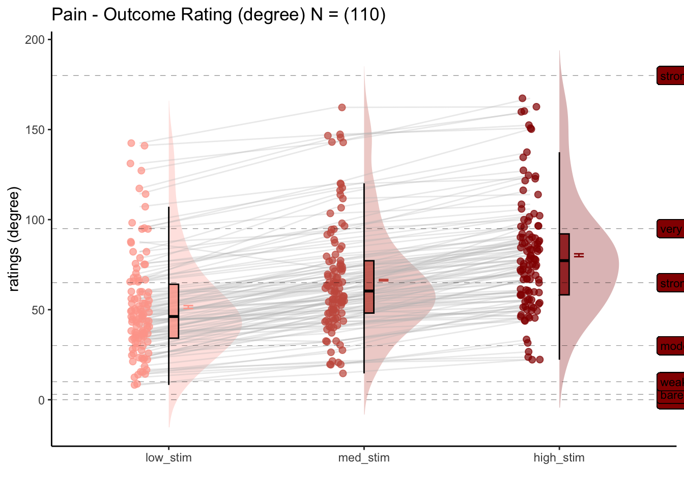
5.2 Vicarious
For the vicarious task, what is the effect of stimulus intensity on outcome ratings?
[ INSERT DESCRIPTION ]
## Warning: Model failed to converge with 1 negative eigenvalue: -8.5e+01## Warning in geom_line(data = subjectwise, aes(group = .data[[subject]], x =
## as.numeric(factor(.data[[iv]])) - : Ignoring unknown aesthetics: fill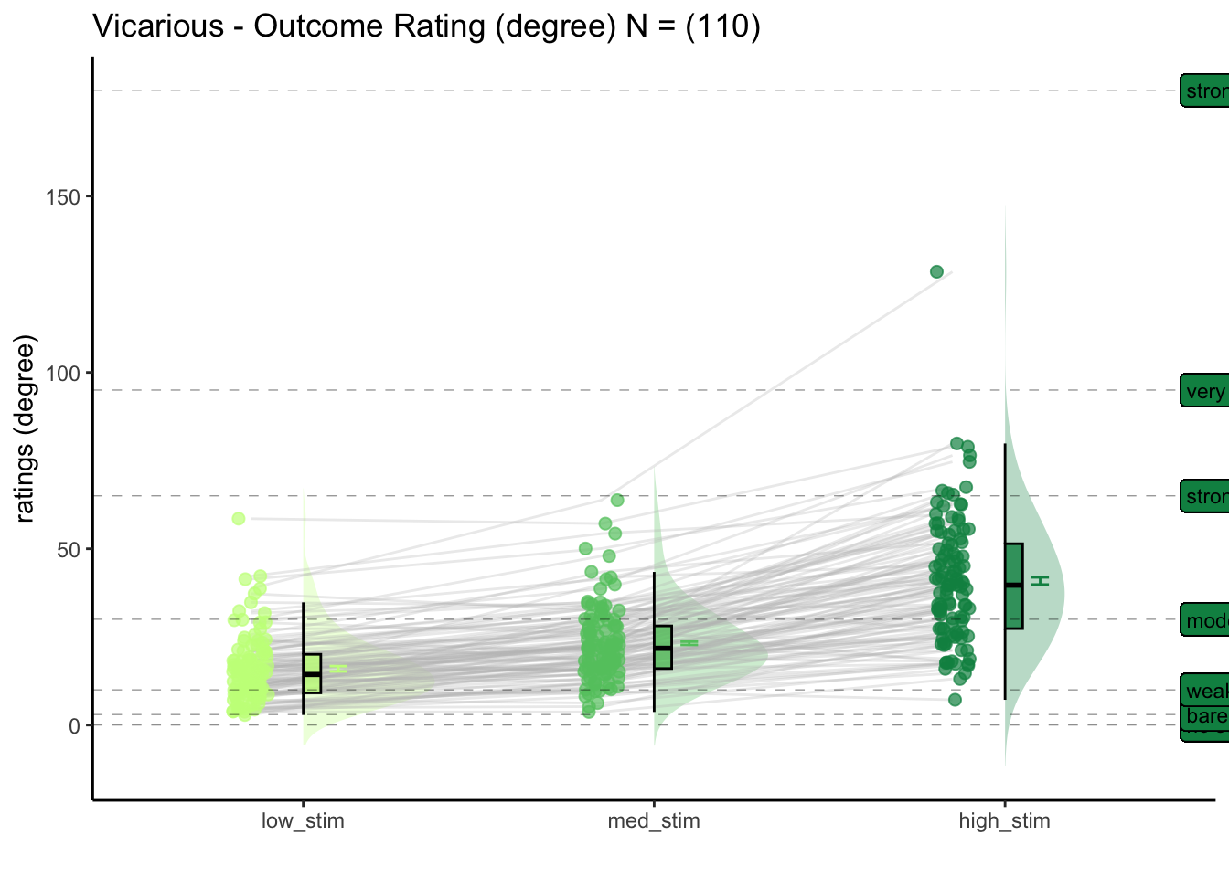
5.3 Cognitive
For the cognitive task, what is the effect of stimulus intensity on outcome ratings?
[ INSERT DESCRIPTION ]
## Warning: Model failed to converge with 1 negative eigenvalue: -1.1e+02## Warning in geom_line(data = subjectwise, aes(group = .data[[subject]], x =
## as.numeric(factor(.data[[iv]])) - : Ignoring unknown aesthetics: fill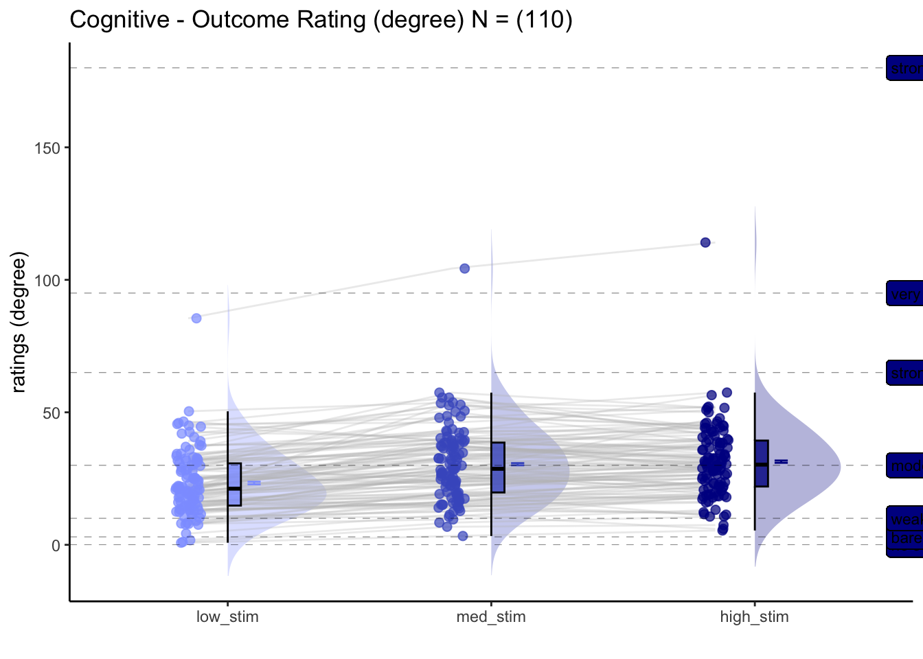
5.4 for loop
combined_se_calc_cooksd <- data.frame()
analysis_dir <- file.path(
        main_dir,
        "analysis", "mixedeffect", "model04_iv-stim_dv-actual",as.character(Sys.Date())
    )
dir.create(analysis_dir, showWarnings = FALSE, recursive = TRUE)

# 1. [ PARAMETERS ]  __________________________________________________ # nolint
dv_keyword <- "actual"
xlab <- ""
ylab <- "judgment (degree)"
for (taskname in c("pain", "vicarious", "cognitive")) {
    ggtitle <- paste(taskname, " - actual judgment (degree)")
    title <- paste(taskname, " - actual")
    subject <- "src_subject_id"
    subject_varkey <- "src_subject_id"
    data <- load_task_social_df(datadir,
        taskname = taskname,
        subject_varkey = "src_subject_id",

        iv = "param_cue_type",
        dv = "event04_actual_angle",
        exclude = "sub-0001|sub-0003|sub-0004|sub-0005|sub-0025|sub-0999"
    )

    w <- 10
    h <- 6

    # [ CONTRASTS ]  ________________________________________________________________________________ # nolint
    # contrast code ________________________________________
    data$stim[data$event03_stimulus_type == "low_stim"] <- -0.5 # social influence task
    data$stim[data$event03_stimulus_type == "med_stim"] <- 0 # no influence task
    data$stim[data$event03_stimulus_type == "high_stim"] <- 0.5 # no influence task

    data$stim_factor <- factor(data$event03_stimulus_type)

    # contrast code 1 linear
    data$stim_con_linear[data$event03_stimulus_type == "low_stim"] <- -0.5
    data$stim_con_linear[data$event03_stimulus_type == "med_stim"] <- 0
    data$stim_con_linear[data$event03_stimulus_type == "high_stim"] <- 0.5

    # contrast code 2 quadratic
    data$stim_con_quad[data$event03_stimulus_type == "low_stim"] <- -0.33
    data$stim_con_quad[data$event03_stimulus_type == "med_stim"] <- 0.66
    data$stim_con_quad[data$event03_stimulus_type == "high_stim"] <- -0.33

    # social cude contrast
    data$social_cue[data$param_cue_type == "low_cue"] <- -0.5 # social influence task
    data$social_cue[data$param_cue_type == "high_cue"] <- 0.5 # no influence task

    stim_con1 <- "stim_con_linear"
    stim_con2 <- "stim_con_quad"
    iv1 <- "param_cue_type"
    #iv1 <- "social_cue"
    dv <- "event04_actual_angle"

    # [ MODEL ] _________________________________________________ # nolint
    model_savefname <- file.path(
        analysis_dir,
        paste("lmer_task-", taskname,
            "_rating-", dv_keyword,
            "_", as.character(Sys.Date()), "_cooksd.txt",
            sep = ""
        )
    )
    cooksd <- lmer_onefactor_cooksd(
        data, taskname, iv, dv,
        subject, dv_keyword, model_savefname, print_lmer_output = TRUE
    )
    influential <- as.numeric(names(cooksd)[
        (cooksd > (4 / as.numeric(length(unique(data$src_subject_id)))))
    ])
    data_screen <- data[-influential, ]
    # [ PLOT ] reordering for plots _________________________ # nolint
    data_screen$stim_name[data_screen$param_stimulus_type == "high_stim"] <- "high"
    data_screen$stim_name[data_screen$param_stimulus_type == "med_stim"] <- "med"
    data_screen$stim_name[data_screen$param_stimulus_type == "low_stim"] <- "low"

    # DATA$levels_ordered <- factor(DATA$param_stimulus_type, levels=c("low", "med", "high"))

    data_screen$stim_ordered <- factor(
        data_screen$stim_name,
        levels = c("low", "med", "high")
    )
    model_iv1 <- "stim_ordered"
    #model_iv2 <- "cue_ordered"

    #  [ PLOT ] calculate mean and se  _________________________
    actual_subjectwise <- meanSummary(
        data_screen,
        c("src_subject_id", model_iv1), dv
    )
    actual_groupwise <- summarySEwithin(
        data = actual_subjectwise,
        measurevar = "mean_per_sub",
        withinvars = c(model_iv1), idvar = "src_subject_id"
    )
    actual_groupwise$task <- taskname
    # https://stackoverflow.com/questions/29402528/append-data-frames-together-in-a-for-loop/29419402
    combined_se_calc_cooksd <- rbind(combined_se_calc_cooksd, actual_groupwise)

    #  [ PLOT ] calculate mean and se  ----------------------------------------------------------------------------
    sub_mean <- "mean_per_sub"
    group_mean <- "mean_per_sub_norm_mean"
    se <- "se"
    subject <- "src_subject_id"
    ggtitle <- paste(taskname, " - Actual Rating (degree) Cooksd removed")
    title <- paste(taskname, " - Actual")
    xlab <- ""
    ylab <- "ratings (degree)"
    ylim <- c(-10,190)
    dv_keyword <- "actual"
    if (any(startsWith(dv_keyword, c("expect", "Expect")))) {
        color <- c("#1B9E77", "#D95F02", "#D95F02")
    } else {
        color <- c("#4575B4", "#D73027", "#D95F02" )
    } # if keyword starts with
    plot_savefname <- file.path(
        analysis_dir,
        paste("raincloud_task-", taskname,
            "_rating-", dv_keyword,
            "_", as.character(Sys.Date()), "_cooksd.png",
            sep = ""
        )
    )
    g <- plot_halfrainclouds_onefactor(
        actual_subjectwise, actual_groupwise, model_iv1,
        sub_mean, group_mean, se, subject,
        ggtitle, title, xlab, ylab, taskname,ylim,
        w, h, dv_keyword, color, plot_savefname
    )

    g <- g +
      geom_hline(yintercept = 0, size = 0.1, linetype = "dashed") +
      geom_label(x = 3.5, y = 0, label = c("no sensation"), hjust = 0, nudge_x = 0.1, size = 3) +
      geom_hline(yintercept = 3, size = 0.1, linetype = "dashed") +
      geom_label(x = 3.5, y = 3, label = c("barely detectable"), hjust = 0, nudge_x = 0.1, size = 3) +
      geom_hline(yintercept = 10, size = 0.1, linetype = "dashed") +
      geom_label(x = 3.5, y = 10, label = c("weak"), hjust = 0, nudge_x = 0.1, size = 3) +
      geom_hline(yintercept = 30, size = 0.1, linetype = "dashed") +
      geom_label(x = 3.5, y = 30, label = c("moderate"), hjust = 0, nudge_x = 0.1, size = 3) +
      geom_hline(yintercept = 65, size = 0.1, linetype = "dashed") +
      geom_label(x = 3.5, y = 65, label = c("strong"), hjust = 0, nudge_x = 0.1, size = 3) +
      geom_hline(yintercept = 95, size = 0.1, linetype = "dashed") +
      geom_label(x = 3.5, y = 95, label = c("very strong"), hjust = 0, nudge_x = 0.1, size = 3) +
      geom_hline(yintercept = 180, size = 0.1, linetype = "dashed") +
      geom_label(x = 3.5, y = 180, label = c("strongest imaginable"), hjust = 0, nudge_x = 0.1, size = 3) +
      coord_cartesian(clip = 'off')+
      theme_classic() +
      theme(legend.position = "none")

    ggsave(plot_savefname, width = w, height = h)

  g

    # save fixed random effects _______________________________
#     randEffect$newcoef <- mapvalues(randEffect$term,
#         from = c("(Intercept)", "data[, iv]",
#                  "data[, stim_con1]", "data[, stim_con2]",
#                  "data[, iv]:data[, stim_con1]",
#                  "data[, iv]:data[, stim_con2]"),
#         to = c("rand_intercept", "rand_cue", "rand_stimlin",
#                "rand_stimquad", "rand_int_cue_stimlin", #"rand_int_cue_stimquad")
#     )
#
#     #
#     # # The arguments to spread():
#     # # - data: Data object
#     # # - key: Name of column containing the new column names
#     # # - value: Name of column containing values
#     #
#     # # TODO: add fixed effects
#     #
#     rand_subset <- subset(randEffect, select = -c(grpvar, term, condsd))
#     wide_rand <- spread(rand_subset, key = newcoef, value = condval)
#     wide_fix <- do.call(
#         "rbind",
#         replicate(nrow(wide_rand), #as.data.frame(t(as.matrix(fixEffect))),
#             simplify = FALSE
#         )
#     )
#     rownames(wide_fix) <- NULL
#     new_wide_fix <- dplyr::rename(wide_fix,
#         fix_intercept = `(Intercept)`,
#         fix_cue = `social_cue`, # `data[, iv]`,
#         fix_stimulus_linear = `stim_con_linear`, # `data[, stim_con1]`,
#         fix_stimulus_quad = `stim_con_quad`, #`data[, stim_con2]`,
#         fix_int_cue_stimlin = `social_cue:stim_con_linear`, #`data[, iv]:data[, stim_con1]`,
#         fix_int_cue_stimquad = `social_cue:stim_con_quad` #`data[, iv]:data[, stim_con2]`
#     )
#
#     total <- cbind(wide_rand, new_wide_fix)
#     total$task <- taskname
#     new_total <- total %>% dplyr::select(task, everything())
#     new_total <- dplyr::rename(total, subj = grp)
#
#     plot_savefname <- file.path(analysis_dir,
#                                 paste("randeffect_task-", taskname,
#                                       "_", as.character(Sys.Date()), #"_outlier-cooksd.csv", sep = ""))
#     write.csv(new_total, plot_savefname, row.names = FALSE)
#
}
## boundary (singular) fit: see help('isSingular')## Linear mixed model fit by REML. t-tests use Satterthwaite's method [
## lmerModLmerTest]
## Formula:
## as.formula(reformulate(c(iv, sprintf("(%s|%s)", iv, subject_keyword)),
## response = dv))
## Data: df
##
## REML criterion at convergence: 52938.5
##
## Scaled residuals:
## Min 1Q Median 3Q Max
## -4.5365 -0.5608 -0.0002 0.5695 4.6143
##
## Random effects:
## Groups Name Variance Std.Dev. Corr
## src_subject_id (Intercept) 952.46 30.862
## param_stimulus_typelow_stim 127.22 11.279 -0.47
## param_stimulus_typemed_stim 29.79 5.458 -0.24 0.97
## Residual 448.14 21.169
## Number of obs: 5851, groups: src_subject_id, 110
##
## Fixed effects:
## Estimate Std. Error df t value Pr(>|t|)
## (Intercept) 80.3242 2.9886 109.1411 26.88 <2e-16 ***
## param_stimulus_typelow_stim -29.2521 1.2974 107.5783 -22.55 <2e-16 ***
## param_stimulus_typemed_stim -13.7621 0.8652 148.5592 -15.90 <2e-16 ***
## ---
## Signif. codes: 0 '***' 0.001 '**' 0.01 '*' 0.05 '.' 0.1 ' ' 1
##
## Correlation of Fixed Effects:
## (Intr) prm_stmls_typl_
## prm_stmls_typl_ -0.455
## prm_stmls_typm_ -0.236 0.718
## optimizer (nloptwrap) convergence code: 0 (OK)
## boundary (singular) fit: see help('isSingular')## Warning in geom_line(data = subjectwise, aes(group = .data[[subject]], x =
## as.numeric(factor(.data[[iv]])) - : Ignoring unknown aesthetics: fill## Coordinate system already present. Adding new coordinate system, which will
## replace the existing one.
## boundary (singular) fit: see help('isSingular')## Linear mixed model fit by REML. t-tests use Satterthwaite's method [
## lmerModLmerTest]
## Formula:
## as.formula(reformulate(c(iv, sprintf("(%s|%s)", iv, subject_keyword)),
## response = dv))
## Data: df
##
## REML criterion at convergence: 56882.7
##
## Scaled residuals:
## Min 1Q Median 3Q Max
## -5.5482 -0.5779 -0.1812 0.4475 6.1884
##
## Random effects:
## Groups Name Variance Std.Dev. Corr
## src_subject_id (Intercept) 283.44 16.836
## param_stimulus_typelow_stim 172.13 13.120 -0.88
## param_stimulus_typemed_stim 98.63 9.931 -0.85 1.00
## Residual 448.25 21.172
## Number of obs: 6313, groups: src_subject_id, 110
##
## Fixed effects:
## Estimate Std. Error df t value Pr(>|t|)
## (Intercept) 40.822 1.681 108.598 24.29 <2e-16 ***
## param_stimulus_typelow_stim -24.936 1.426 109.210 -17.49 <2e-16 ***
## param_stimulus_typemed_stim -17.614 1.162 114.541 -15.15 <2e-16 ***
## ---
## Signif. codes: 0 '***' 0.001 '**' 0.01 '*' 0.05 '.' 0.1 ' ' 1
##
## Correlation of Fixed Effects:
## (Intr) prm_stmls_typl_
## prm_stmls_typl_ -0.837
## prm_stmls_typm_ -0.784 0.862
## optimizer (nloptwrap) convergence code: 0 (OK)
## boundary (singular) fit: see help('isSingular')## Warning in geom_line(data = subjectwise, aes(group = .data[[subject]], x =
## as.numeric(factor(.data[[iv]])) - : Ignoring unknown aesthetics: fill## Coordinate system already present. Adding new coordinate system, which will
## replace the existing one.
## boundary (singular) fit: see help('isSingular')## Linear mixed model fit by REML. t-tests use Satterthwaite's method [
## lmerModLmerTest]
## Formula:
## as.formula(reformulate(c(iv, sprintf("(%s|%s)", iv, subject_keyword)),
## response = dv))
## Data: df
##
## REML criterion at convergence: 54866.8
##
## Scaled residuals:
## Min 1Q Median 3Q Max
## -3.7173 -0.6283 -0.1660 0.4545 7.0548
##
## Random effects:
## Groups Name Variance Std.Dev. Corr
## src_subject_id (Intercept) 176.9233 13.3013
## param_stimulus_typelow_stim 8.2230 2.8676 -0.75
## param_stimulus_typemed_stim 0.4181 0.6466 0.37 0.33
## Residual 374.7596 19.3587
## Number of obs: 6220, groups: src_subject_id, 110
##
## Fixed effects:
## Estimate Std. Error df t value Pr(>|t|)
## (Intercept) 31.4642 1.3417 109.5625 23.451 <2e-16 ***
## param_stimulus_typelow_stim -8.1551 0.6623 106.7910 -12.313 <2e-16 ***
## param_stimulus_typemed_stim -1.0096 0.6056 718.4229 -1.667 0.0959 .
## ---
## Signif. codes: 0 '***' 0.001 '**' 0.01 '*' 0.05 '.' 0.1 ' ' 1
##
## Correlation of Fixed Effects:
## (Intr) prm_stmls_typl_
## prm_stmls_typl_ -0.500
## prm_stmls_typm_ -0.186 0.465
## optimizer (nloptwrap) convergence code: 0 (OK)
## boundary (singular) fit: see help('isSingular')## Warning in geom_line(data = subjectwise, aes(group = .data[[subject]], x =
## as.numeric(factor(.data[[iv]])) - : Ignoring unknown aesthetics: fill## Coordinate system already present. Adding new coordinate system, which will
## replace the existing one.5.5 Lineplot
library(ggpubr)
DATA = as.data.frame(combined_se_calc_cooksd)
color = c( "#4575B4", "#D73027")
LINEIV1 = "stim_ordered"
LINEIV2 = "cue_ordered"
MEAN = "mean_per_sub_norm_mean"
ERROR = "se"
dv_keyword = "actual"
p1 = plot_lineplot_onefactor(DATA, 'pain',
               LINEIV1, MEAN, ERROR, color, xlab = "Stimulus intensity" , ylab= "Outcome rating", ggtitle = 'pain' )
p2 = plot_lineplot_onefactor(DATA,'vicarious',
               LINEIV1, MEAN, ERROR, color,xlab = "Stimulus intensity" , ylab= "Outcome rating",ggtitle = 'vicarious')
p3 = plot_lineplot_onefactor(DATA, 'cognitive',
               LINEIV1, MEAN, ERROR, color,xlab = "Stimulus intensity" , ylab= "Outcome rating",ggtitle = 'cognitive')
#grid.arrange(p1, p2, p3, ncol=3 , common.legend = TRUE)
ggpubr::ggarrange(p1,p2,p3,ncol = 3, nrow = 1, common.legend = TRUE,legend = "bottom")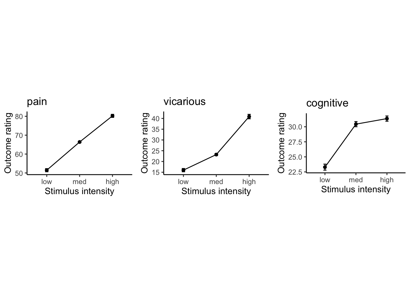
plot_filename = file.path(analysis_dir,
                          paste('lineplot_task-all_rating-',dv_keyword,'.png', sep = ""))
ggsave(plot_filename, width = 15, height = 6)