Chapter 13 (N-2) shifted outcome ratings ~ (N) expectation ratings; Jayazeri (2018)
title: "model12_jayazeri_N-2"
date: '2023-01-31'
updated: '2023-01-31'
Overview
My hypothesis is that the cue-expectancy follows a Bayesian mechanism, akin to what’s listed in Jayazeri (2019). Here, I plot the expectation ratings (N) and outcome ratings (N-2) and see if the pattern is similar to a sigmoidal curve. If so, I plan to dive deeper and potentially take a Bayesian approach.
library
load data and combine participant data
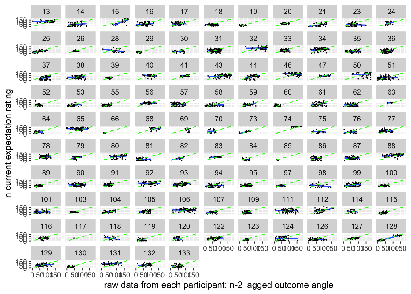
13.1 Do previous outcome ratings predict current expectation ratings?
Additional analyse 01/18/2023
- examine if prior stimulus experience (N-2) predicts current expectation ratings
- see if current expectation ratings are explained as a function of prior outcome rating and current expectation rating
when loading the dataset, I need to add in trial index per dataframe. Then, for the shift the rating?
## Linear mixed model fit by REML. t-tests use Satterthwaite's method [
## lmerModLmerTest]
## Formula: event02_expect_angle ~ lag.04outcomeangle + (1 | src_subject_id) +
##     (1 | session_id)
##    Data: data_a3lag_omit
##
## REML criterion at convergence: 41892
##
## Scaled residuals:
##     Min      1Q  Median      3Q     Max
## -4.7836 -0.6742  0.0243  0.6639  3.4522
##
## Random effects:
##  Groups         Name        Variance Std.Dev.
##  src_subject_id (Intercept) 522.8    22.86
##  session_id     (Intercept)   0.0     0.00
##  Residual                   770.0    27.75
## Number of obs: 4381, groups:  src_subject_id, 104; session_id, 3
##
## Fixed effects:
##                     Estimate Std. Error        df t value Pr(>|t|)
## (Intercept)        4.753e+01  2.548e+00 1.436e+02   18.66   <2e-16 ***
## lag.04outcomeangle 2.343e-01  1.675e-02 4.294e+03   13.98   <2e-16 ***
## ---
## Signif. codes:  0 '***' 0.001 '**' 0.01 '*' 0.05 '.' 0.1 ' ' 1
##
## Correlation of Fixed Effects:
##             (Intr)
## lg.04tcmngl -0.433
## optimizer (nloptwrap) convergence code: 0 (OK)
## boundary (singular) fit: see help('isSingular')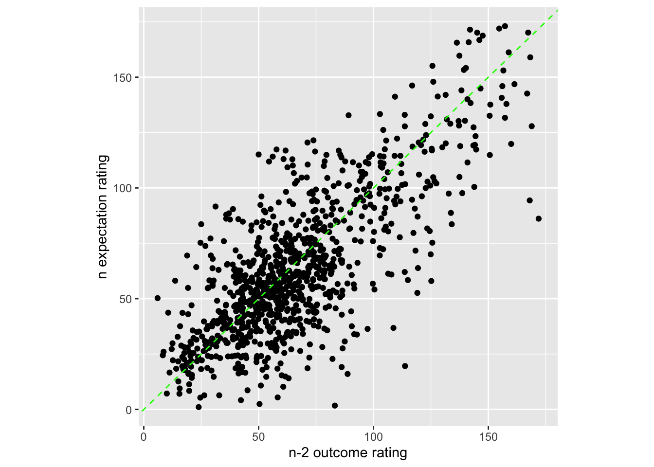
    trialorder_groupwise <- summarySEwithin(
        data = subjectwise_naomit_2dv,
        measurevar = "DV1_mean_per_sub",
        # betweenvars = "src_subject_id",
        withinvars = factor( "trial_index"),
         idvar = "src_subject_id"
    )
## Automatically converting the following non-factors to factors: src_subject_id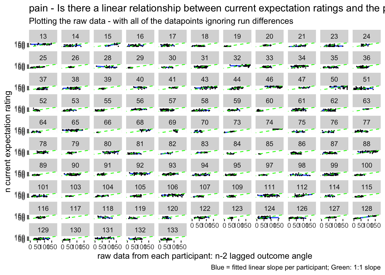
 Warning: Removed 222 rows containing non-finite values (
stat_smooth()).
# https://gist.github.com/even4void/5074855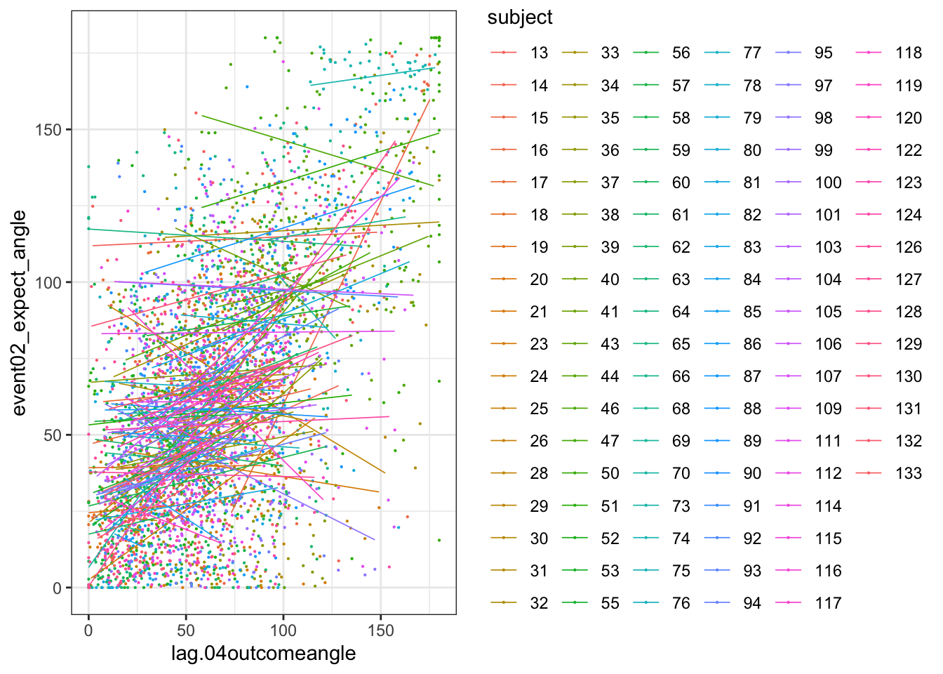 Warning: Removed 222 rows containing non-finite values (
stat_smooth()).
13.2 Do these models differ as a function of cue?
Additional analysis 01/23/2023
## Linear mixed model fit by REML. t-tests use Satterthwaite's method [
## lmerModLmerTest]
## Formula: event02_expect_angle ~ lag.04outcomeangle * param_cue_type +
##     (1 | src_subject_id) + (1 | session_id)
##    Data: data_a3lag_omit
##
## REML criterion at convergence: 39852.4
##
## Scaled residuals:
##     Min      1Q  Median      3Q     Max
## -5.2141 -0.6403 -0.0326  0.6247  4.6722
##
## Random effects:
##  Groups         Name        Variance Std.Dev.
##  src_subject_id (Intercept) 540.1    23.24
##  session_id     (Intercept)   0.0     0.00
##  Residual                   477.4    21.85
## Number of obs: 4381, groups:  src_subject_id, 104; session_id, 3
##
## Fixed effects:
##                                            Estimate Std. Error         df
## (Intercept)                               6.478e+01  2.572e+00  1.495e+02
## lag.04outcomeangle                        2.255e-01  1.631e-02  4.374e+03
## param_cue_typelow_cue                    -3.367e+01  1.346e+00  4.274e+03
## lag.04outcomeangle:param_cue_typelow_cue -3.175e-03  1.771e-02  4.274e+03
##                                          t value Pr(>|t|)
## (Intercept)                               25.186   <2e-16 ***
## lag.04outcomeangle                        13.831   <2e-16 ***
## param_cue_typelow_cue                    -25.025   <2e-16 ***
## lag.04outcomeangle:param_cue_typelow_cue  -0.179    0.858
## ---
## Signif. codes:  0 '***' 0.001 '**' 0.01 '*' 0.05 '.' 0.1 ' ' 1
##
## Correlation of Fixed Effects:
##             (Intr) lg.04t prm___
## lg.04tcmngl -0.418
## prm_c_typl_ -0.273  0.503
## lg.04tc:___  0.243 -0.578 -0.871
## optimizer (nloptwrap) convergence code: 0 (OK)
## boundary (singular) fit: see help('isSingular')
## `geom_smooth()` using formula = 'y ~ x'## Warning: Removed 29 rows containing non-finite values (`stat_smooth()`).## Warning: Removed 29 rows containing missing values (`geom_point()`).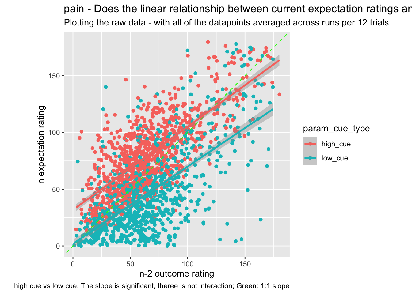
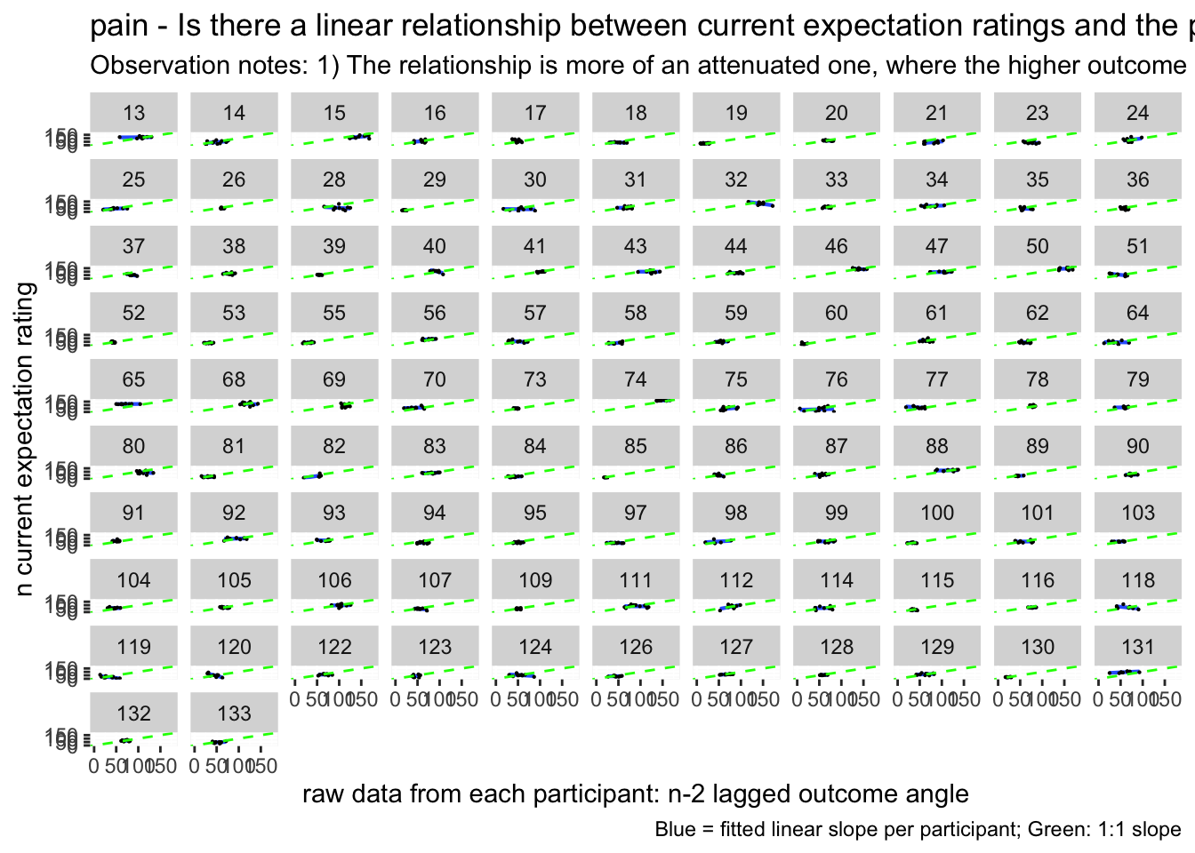
Let’s demean the ratings.
bin ratings Do the bins do their jobs? plot one run then check the min, max and see if the quantization is done properly. YES, it is
# per subject, session, run
df_subset = subset(data_a3lag_omit, src_subject_id == 18 )
#df_subset$lag.04outcomeangle
min(df_subset$lag.04outcomeangle)
## [1] 0max(df_subset$lag.04outcomeangle)## [1] 88.7054range(df_subset$lag.04outcomeangle)## [1] 0.0000 88.7054cut_interval(range(df_subset$lag.04outcomeangle), n = 5)## [1] [0,17.7] (71,88.7]
## Levels: [0,17.7] (17.7,35.5] (35.5,53.2] (53.2,71] (71,88.7]hist(df_subset$lag.04outcomeangle)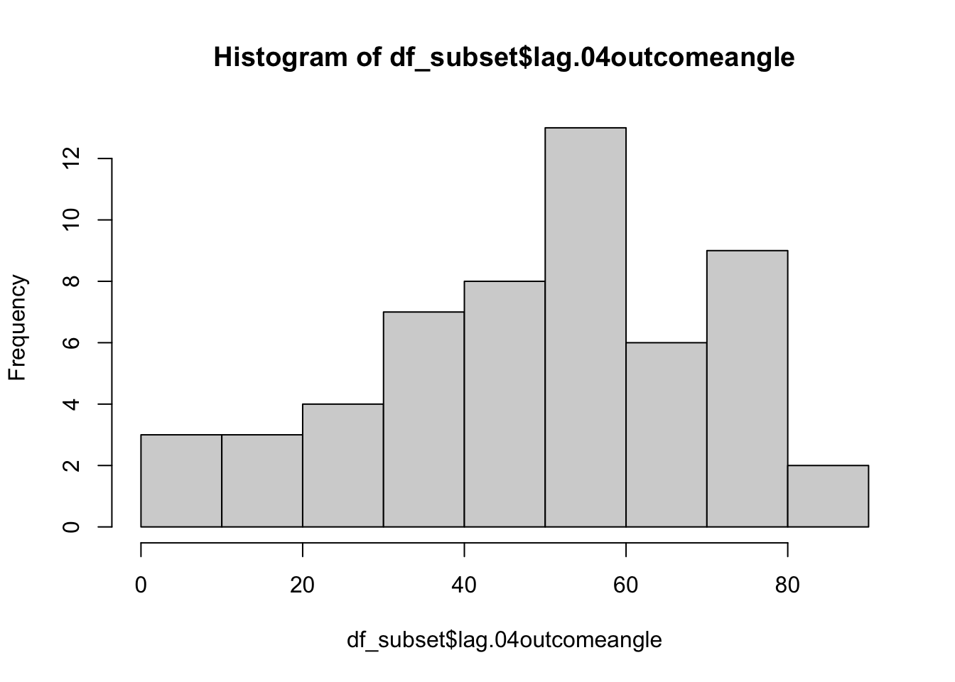
df_subset$bin = cut_interval(df_subset$lag.04outcomeangle, n = 5)
df_subset$bin_num = as.numeric(cut_interval(df_subset$lag.04outcomeangle, n = 5))
df_discrete = data_a3lag_omit %>%
group_by(src_subject_id) %>%
mutate(bin = cut_interval(lag.04outcomeangle, n = 5),
n_2outcomelevels = as.numeric(cut_interval(lag.04outcomeangle, n = 5)))13.2.1 confirm that df discrete has 5 levels per participant
the number of counts per frequency can differ
res <- df_discrete %>%
  group_by(src_subject_id,n_2outcomelevels) %>%
tally()res## # A tibble: 514 × 3
## # Groups: src_subject_id [104]
## src_subject_id n_2outcomelevels n
## <fct> <dbl> <int>
## 1 13 1 1
## 2 13 2 4
## 3 13 3 4
## 4 13 4 12
## 5 13 5 19
## 6 14 1 10
## 7 14 2 16
## 8 14 3 7
## 9 14 4 6
## 10 14 5 1
## # … with 504 more rowspain_df = df_discrete[df_discrete$param_task_name == "pain",]
ggplot(pain_df, aes(y = event02_expect_angle,
x = n_2outcomelevels,
colour = subject), size = .3, color = 'gray') +
geom_point(size = .1) +
geom_smooth(method = "gam") +
theme_bw()## `geom_smooth()` using formula = 'y ~ s(x, bs = "cs")'## Warning: Removed 202 rows containing non-finite values (`stat_smooth()`).## Warning: Computation failed in `stat_smooth()`
## Caused by error in `smooth.construct.cr.smooth.spec()`:
## ! x has insufficient unique values to support 10 knots: reduce k.## Warning: Removed 202 rows containing missing values (`geom_point()`).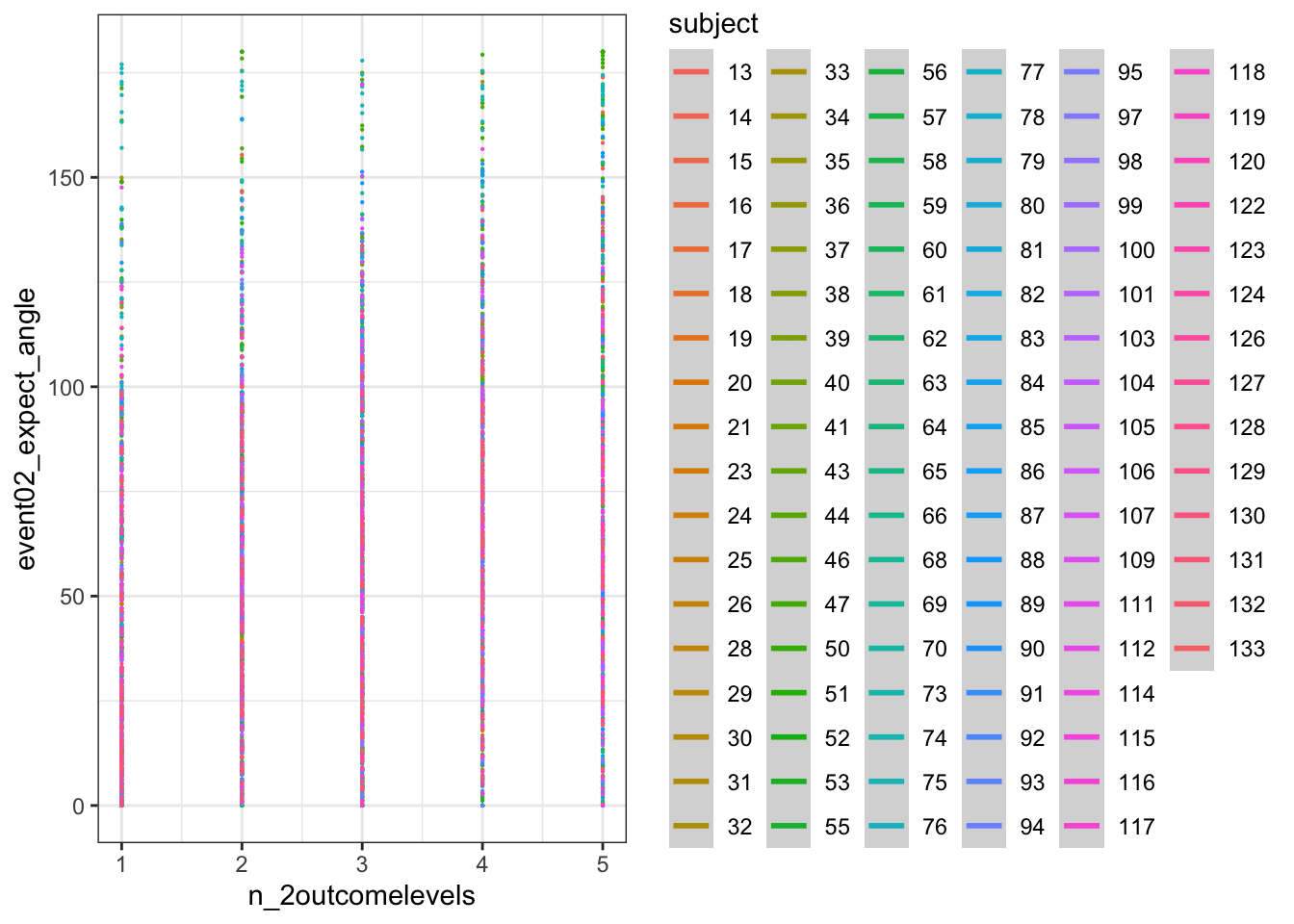
13.3 Demean and discretize
df_discrete = data_a3lag_omit %>%
  group_by(src_subject_id) %>%
  mutate(lag.04outcomeangle_demean = lag.04outcomeangle-mean(lag.04outcomeangle),
         event02_expect_angle_demean = event02_expect_angle-mean(event02_expect_angle)) %>%
  mutate(bin = cut_interval(lag.04outcomeangle_demean, n = 5),
         n_2outcomelevels = as.numeric(cut_interval(lag.04outcomeangle_demean, n = 5)))
Check how many trials land in each outcome level
res <- df_discrete %>%
  group_by(src_subject_id,n_2outcomelevels) %>%
  tally()
res
## # A tibble: 514 × 3
## # Groups: src_subject_id [104]
## src_subject_id n_2outcomelevels n
## <fct> <dbl> <int>
## 1 13 1 1
## 2 13 2 4
## 3 13 3 4
## 4 13 4 12
## 5 13 5 19
## 6 14 1 10
## 7 14 2 16
## 8 14 3 7
## 9 14 4 6
## 10 14 5 1
## # … with 504 more rowspain_df = df_discrete[df_discrete$param_task_name == "pain",]
ggplot(pain_df, aes(y = event02_expect_angle_demean,
x = n_2outcomelevels,
colour = subject), size = .3, color = 'gray') +
geom_point(size = .1) +
geom_smooth(method = "gam") +
theme_bw()## `geom_smooth()` using formula = 'y ~ s(x, bs = "cs")'## Warning: Removed 2601 rows containing non-finite values (`stat_smooth()`).## Warning: Computation failed in `stat_smooth()`
## Caused by error in `smooth.construct.cr.smooth.spec()`:
## ! x has insufficient unique values to support 10 knots: reduce k.## Warning: Removed 2601 rows containing missing values (`geom_point()`).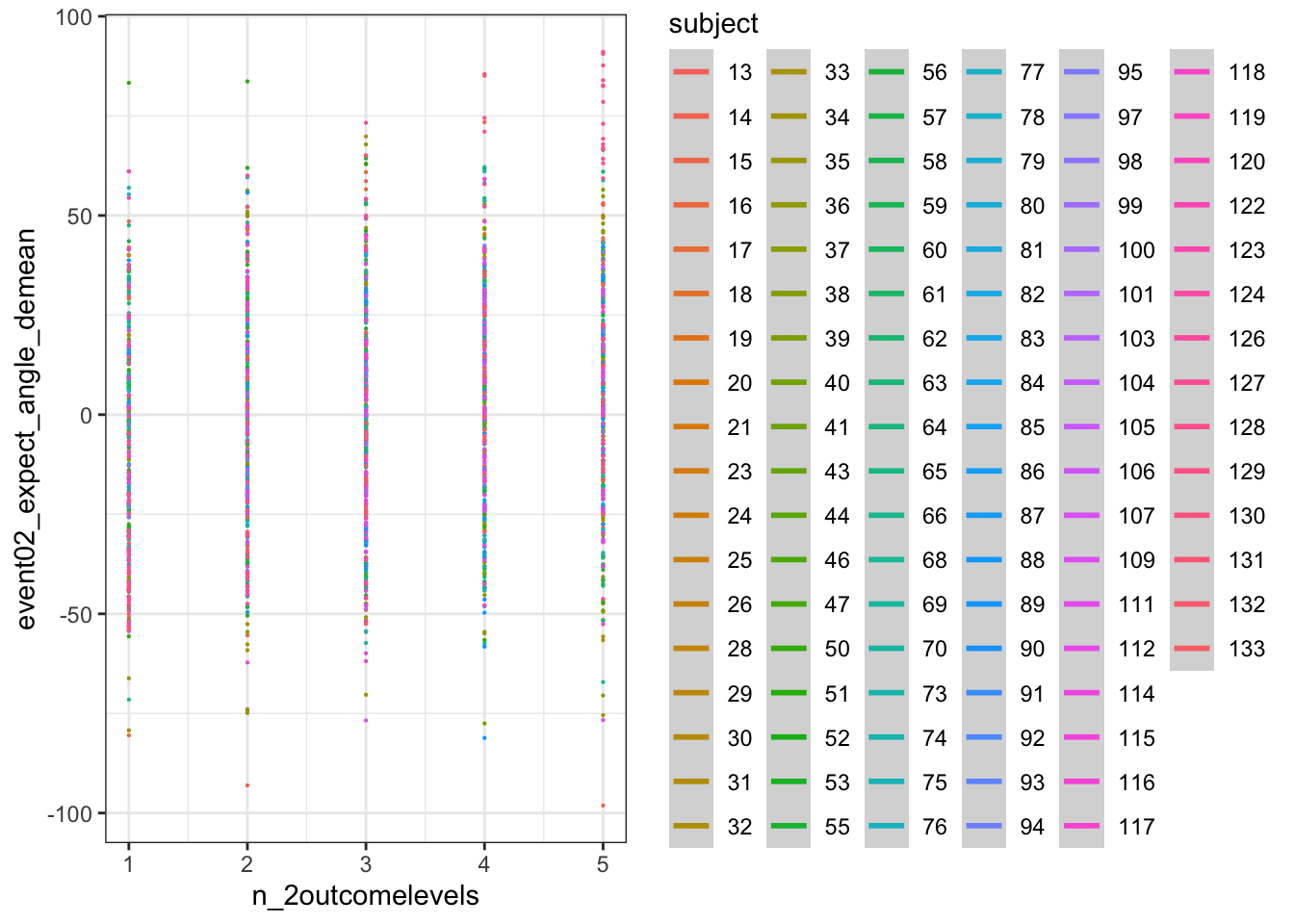
df_discrete$n_2outcomelevels_newlev = df_discrete$n_2outcomelevels -3
    subjectwise_bin_demean <- meanSummary(df_discrete, c(
        "subject","param_task_name","n_2outcomelevels"
    ), "event02_expect_angle_demean")
subjectwise_bin_demean_naomit <- na.omit(subjectwise_bin_demean)
    groupwise_bin_demean <- summarySEwithin(
        data = subjectwise_bin_demean_naomit,
        measurevar = "mean_per_sub", # variable created from above
        withinvars = c("n_2outcomelevels"), # iv
       idvar = "subject"
    )
## Automatically converting the following non-factors to factors: n_2outcomelevelssubjectwise_bin_demean_naomit$n_2outcomelevels_newlev = as.numeric(subjectwise_bin_demean_naomit$n_2outcomelevels) -3
groupwise_bin_demean$n_2outcomelevels_newlev = as.numeric(groupwise_bin_demean$n_2outcomelevels) -3plot_halfrainclouds_sig <- function(subjectwise, groupwise, iv,sub_iv,
subjectwise_mean, group_mean, se, subject,
ggtitle, title, xlab, ylab, taskname, ylim,
w, h, dv_keyword, color, save_fname) {
g <- ggplot(
data = subjectwise,
aes(
y = .data[[subjectwise_mean]],
x = factor(.data[[iv]]),
fill = factor(.data[[iv]])
)
) +
coord_cartesian(ylim = ylim, expand = TRUE) +
geom_half_violin(
aes(fill = factor(.data[[iv]])),
side = 'r',
#position = 'dodge',
adjust = 0.5,
trim = FALSE,
alpha = .5,
colour = NA
) +
geom_point(
aes(
# group = .data[[subject]],
x = as.numeric(factor(.data[[iv]])) - .1 ,
y = .data[[subjectwise_mean]],
color = factor(.data[[iv]])
),
position = position_jitter(width = .05),
size = 2,
alpha = 0.7,
) +
geom_errorbar(
data = groupwise,
aes(
x = as.numeric(.data[[sub_iv]]) + .1 ,
y = as.numeric(.data[[group_mean]]),
color = factor(.data[[iv]]),
ymin = .data[[group_mean]] - .data[[se]],
ymax = .data[[group_mean]] + .data[[se]]
),
position = position_dodge(width=0.1), width=0.1 , # position = 'dodge',
alpha = 1
) +
geom_line(
data = groupwise,
aes(
#group = .data[[subject]],
group = 1,
y = as.numeric(.data[[group_mean]]),
x = as.numeric(.data[[sub_iv]]) + .1 ,
# fill = factor(.data[[iv]])
),
linetype = "solid", color = "#C97482", alpha = 1
) +
# legend stuff ________________________________________________________ # nolint
guides(color = "none") +
guides(fill = guide_legend(title = title)) +
scale_fill_manual(values = color) +
scale_color_manual(values = color) +
ggtitle(ggtitle) +
xlab(xlab) +
ylab(ylab) +
theme_bw()
ggsave(save_fname, width = w, height = h)
return(g)
}df_discrete$n_2outcomelevels_newlev = as.factor(df_discrete$n_2outcomelevels_newlev)
g <-
plot_halfrainclouds_sig(
subjectwise_bin_demean_naomit,
groupwise_bin_demean,
iv = "n_2outcomelevels_newlev",
sub_iv = "n_2outcomelevels",
subjectwise_mean = "mean_per_sub",
group_mean = "mean_per_sub_norm_mean",
se = "se",
subject = "subject",
ggtitle = "Do we see a sigmoidal pattern in the pain task?\nPrevious outcome ratings predict expectation ratings",
title = "levels of (N-2) outcome ratings",
xlab = "outcome ratings (N-2)",
ylab = "expectation ratings (N)",
taskname = "pain",
ylim = c(-40, 40),
w = 3,
h = 5,
dv_keyword = "sigmoidal",
color = c(
'#ad2831',
"#800e13",
"#640d14",
"#38040e",
"#250902",
"#250902"
),
save_fname = "~/Download/TEST_n-2.png"
)
g https://groups.google.com/g/ggplot2/c/csPNfSLKkco
g +    geom_errorbar(
      data = groupwise_bin_demean,
      aes(
        x = as.numeric("n_2outcomelevels_newlev")  ,
        y = as.numeric("mean_per_sub_norm_mean"),
        #colour = as.numeric("n_2outcomelevels_newlev"),
        ymin = mean_per_sub_norm_mean - se,
        ymax = mean_per_sub_norm_mean + se
      ), width = .1    )
## Warning in FUN(X[[i]], ...): NAs introduced by coercion
## Warning in FUN(X[[i]], ...): NAs introduced by coercion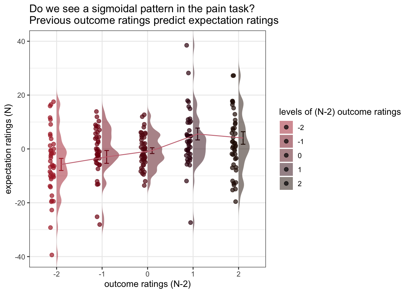
g