Chapter 6 outcome_rating ~ cue * stim

6.1 What is the purpose of this notebook?

Here, I plot the outcome ratings as a function of cue and stimulus intensity. * Main model: lmer(outcome_rating ~ cue * stim) * Main question: do outcome ratings differ as a function of cue type and stimulus intensity? * If there is a main effect of cue on outcome ratings, does this cue effect differ depending on task type? * Is there an interaction between the two factors? * IV: - cue (high / low) - stim (high / med / low) * DV: outcome rating

6.2 model 03 iv-cuecontrast dv-actual

## common dir for saving plots and model outputs
analysis_dir <- file.path(
    main_dir, "analysis",
    "mixedeffect", "model04_iv-cuecontrast_dv-outcome", as.character(Sys.Date()))
dir.create(analysis_dir, recursive = TRUE, showWarnings = FALSE)

for (taskname in c("pain", "vicarious", "cognitive")) {
    subject_varkey <- "src_subject_id"
    iv <- "param_cue_type"; iv_keyword <- "cue"
    dv <- "event04_actual_angle"
    dv_keyword <- "actual"
    subject <- "subject"
    xlab <- ""
    ylab <- "ratings (degree)"
    exclude <- "sub-0001|sub-0003|sub-0004|sub-0005|sub-0025|sub-0999"
    w <- 10
    h <- 6
    model_savefname <- file.path(
        analysis_dir,
        paste("lmer_task-", taskname, "_cue_on_rating-", dv_keyword, "_",
            as.character(Sys.Date()), ".txt",
            sep = ""
        )
    )
    # ___ 1) load data _______________________________________________________________ # nolint
    data <- load_task_social_df(datadir, taskname, subject_varkey, iv, dv, exclude)
    unique(data$src_subject_id)
    data$subject <- factor(data$src_subject_id)

    # ___ 2) mixed effects model _____________________________________________________ # nolint
    cooksd <- lmer_onefactor_cooksd(
        df = data, taskname, iv, dv, subject_keyword = subject, dv_keyword, model_savefname, print_lmer_output=FALSE
    )
    influential <- as.numeric(names(cooksd)[
        (cooksd > (4 / as.numeric(length(unique(data$subject)))))
    ])
    data_screen <- data[-influential, ]

    # ___ 3) calculate difference scores and summarize _______________________________ # nolint
    # TODO: within param_run_num
    data$run_order[data$param_run_num > 3] <- "a"
    data$run_order[data$param_run_num <= 3] <- "b"
    sub_diff <- subset(data, select = c(
        "subject", "session_id", "run_order",
        "param_task_name", "param_cue_type",
        "param_stimulus_type", dv
    ))
    subjectwise <- meanSummary(sub_diff, c(
        "subject", "session_id", "run_order",
        "param_task_name", "param_cue_type",
        "param_stimulus_type"
    ), dv)
    mean_actual <- subjectwise[1:(length(subjectwise) - 1)]
    wide <- mean_actual %>%
        spread(param_cue_type, mean_per_sub)
    wide$diff <- wide$high_cue - wide$low_cue
    wide$stim_name[wide$param_stimulus_type == "high_stim"] <- "high"
    wide$stim_name[wide$param_stimulus_type == "med_stim"] <- "med"
    wide$stim_name[wide$param_stimulus_type == "low_stim"] <- "low"
    wide$stim_ordered <- factor(wide$stim_name,
        levels = c("low", "med", "high")
    )

    subjectwise_diff <- meanSummary(wide, c("subject", "stim_ordered"), "diff")
    subjectwise_diff$stim_ordered <- factor(subjectwise_diff$stim_ordered,
        levels = c("low", "med", "high")
    )
    groupwise_diff <- summarySEwithin(
        data = subjectwise_diff,
        measurevar = "mean_per_sub", # variable created from above
        withinvars = c("stim_ordered"), # iv
        idvar = "subject"
    )

    # ___ 4) plot ____________________________________________________________________  # nolint
    # 4-1. parameters ______________________________________________________________ # nolint
    subjectwise <- subjectwise_diff
    groupwise <- groupwise_diff
    iv <- "stim_ordered"
    subject_mean <- "mean_per_sub"
    group_mean <- "mean_per_sub_norm_mean"
    p1.se <- "se"
    subject <- "subject"
    if (any(startsWith(taskname, c("pain", "Pain")))) { # red
        color <- c("#B7021E", "#B7021E", "#B7021E")
    } else if (any(startsWith(taskname, c("vicarious", "Vicarious")))) { # green
        color <- c("#22834A", "#22834A", "#22834A")
    } else if (any(startsWith(taskname, c("cognitive", "Cognitive")))) { # blue
        color <- c("#0237C9", "#0237C9", "#0237C9")
    }

    # 4-2. plot rain cloud plots ____________________________________________________ # nolint
    p1.xlab <- ""
    p1.ylab <- "Cue effect \n(actual ratings of high > low cue)"
    ylim <- c()
    p1.ggtitle <- paste(taskname, " - actual judgment (degree)")
    p1.title <- paste(taskname, " - actual")
    p1.save_fname <- file.path(
        analysis_dir,
        paste("raincloud_task-", taskname, "_rating-",
            dv_keyword, "-cuecontrast_", as.character(Sys.Date()), ".png",
            sep = ""
        )
    )
    dv_keyword = "cuecontrast"
    ylim = c(-75,75)
    g <- plot_rainclouds_onefactor(
        subjectwise, groupwise, iv, subject_mean, group_mean, p1.se,
        subject, p1.ggtitle, p1.title, p1.xlab, p1.ylab, taskname, ylim,
        w, h, dv_keyword, color, p1.save_fname
    )
    g <- g + geom_hline(yintercept = 0, size = 0.5, linetype = "dashed")
    ggsave(p1.save_fname, plot = g)

    # 4-3.  plot geom range _________________________________________________________ # nolint
    p2.se <- "sd" # se, sd, ci
    p2.xlab <- "stimulus intensity"
    p2.ylab <- "Cue effect \n(actual ratings of high > low cue)"
    p2.ggtitle <- paste(taskname, " - cue effect per stimulus intensity", sep = "")
    w <- 5
    h <- 5
    p2.save_fname <- file.path(
        analysis_dir,
        paste("cueeffect_task-", taskname, "_rating-", dv_keyword, "_",
            as.character(Sys.Date()), ".png",
            sep = ""
        )
    )
    r <- plot_geompointrange_onefactor(
        subjectwise, groupwise, iv,
        subject_mean, group_mean, p2.se,
        p2.xlab, p2.ylab, color, p2.ggtitle, w, h, p2.save_fname
    )
    r <- r + geom_hline(yintercept = 0, size = 1, linetype = "dashed")
    ggsave(p2.save_fname, plot = r)
}

## Warning in geom_line(data = subjectwise, aes(group = .data[[subject]], y
## = .data[[subjectwise_mean]], : Ignoring unknown aesthetics: fill

## Warning: Removed 1 rows containing non-finite values (`stat_ydensity()`).

## Warning: Removed 1 rows containing non-finite values (`stat_boxplot()`).

## Warning: Using the `size` aesthietic with geom_polygon was deprecated in ggplot2 3.4.0.
## ℹ Please use the `linewidth` aesthetic instead.

## Warning: Removed 1 row containing missing values (`geom_line()`).

## Warning: Removed 1 rows containing missing values (`geom_point()`).

## Warning: Using `size` aesthetic for lines was deprecated in ggplot2 3.4.0.
## ℹ Please use `linewidth` instead.

## Saving 7 x 5 in image

## Warning: Removed 1 rows containing non-finite values (`stat_ydensity()`).

## Warning: Removed 1 rows containing non-finite values (`stat_boxplot()`).

## Warning: Removed 1 row containing missing values (`geom_line()`).

## Warning: Removed 1 rows containing missing values (`geom_point()`).

## Warning: The `<scale>` argument of `guides()` cannot be `FALSE`. Use "none" instead as
## of ggplot2 3.3.4.

## Saving 7 x 5 in image

## Warning: Removed 1 rows containing missing values (`geom_point()`).

## Warning: Removed 3 rows containing missing values (`geom_pointrange()`).

## Warning in geom_line(data = subjectwise, aes(group = .data[[subject]], y
## = .data[[subjectwise_mean]], : Ignoring unknown aesthetics: fill

## Warning: Removed 1 rows containing non-finite values (`stat_ydensity()`).

## Warning: Removed 1 rows containing non-finite values (`stat_boxplot()`).

## Warning: Removed 1 rows containing missing values (`geom_point()`).

## Saving 7 x 5 in image

## Warning: Removed 1 rows containing non-finite values (`stat_ydensity()`).

## Warning: Removed 1 rows containing non-finite values (`stat_boxplot()`).

## Warning: Removed 1 rows containing missing values (`geom_point()`).

## Saving 7 x 5 in image

## Warning: Removed 1 rows containing missing values (`geom_point()`).

## Warning: Removed 3 rows containing missing values (`geom_pointrange()`).

## Warning in geom_line(data = subjectwise, aes(group = .data[[subject]], y
## = .data[[subjectwise_mean]], : Ignoring unknown aesthetics: fill

## Saving 7 x 5 in image
## Saving 7 x 5 in image

r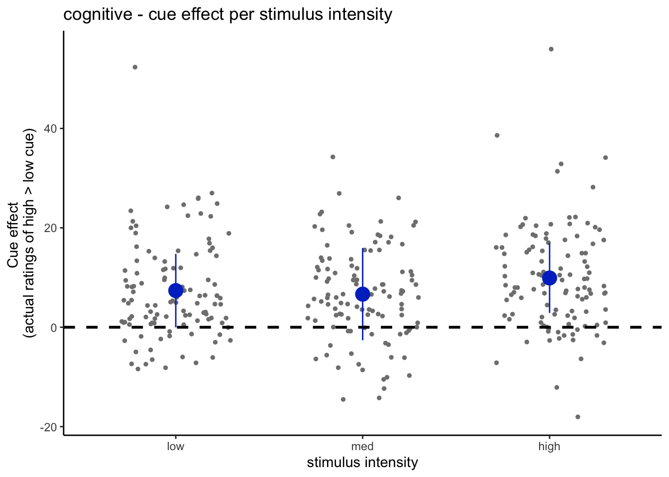

6.2.1 model 03 3-2. individual difference

6.2.2 model 04 iv-cue-stim dv-actual

combined_se_calc_cooksd <- data.frame()
analysis_dir <- file.path(
        main_dir,
        "analysis", "mixedeffect", "model05_iv-cue-stim_dv-actual",as.character(Sys.Date())
    )
dir.create(analysis_dir, showWarnings = FALSE, recursive = TRUE)

# 1. [ PARAMETERS ]  __________________________________________________ # nolint
dv_keyword <- "actual"
xlab <- ""
ylab <- "judgment (degree)"
for (taskname in c("pain", "vicarious", "cognitive")) {
    ggtitle <- paste(taskname, " - actual judgment (degree)")
    title <- paste(taskname, " - actual")
    subject <- "subject"

    data <- load_task_social_df(datadir, 
        taskname = taskname,
        subject_varkey = "src_subject_id",
        iv = "param_cue_type",
        dv = "event04_actual_angle",
        exclude = "sub-0001|sub-0003|sub-0004|sub-0005|sub-0025|sub-0999"
    )

    w <- 10
    h <- 6

    # [ CONTRASTS ]  ________________________________________________________________________________ # nolint
    # contrast code ________________________________________
    data$stim[data$event03_stimulus_type == "low_stim"] <- -0.5 # social influence task
    data$stim[data$event03_stimulus_type == "med_stim"] <- 0 # no influence task
    data$stim[data$event03_stimulus_type == "high_stim"] <- 0.5 # no influence task

    data$stim_factor <- factor(data$event03_stimulus_type)

    # contrast code 1 linear
    data$stim_con_linear[data$event03_stimulus_type == "low_stim"] <- -0.5
    data$stim_con_linear[data$event03_stimulus_type == "med_stim"] <- 0
    data$stim_con_linear[data$event03_stimulus_type == "high_stim"] <- 0.5

    # contrast code 2 quadratic
    data$stim_con_quad[data$event03_stimulus_type == "low_stim"] <- -0.33
    data$stim_con_quad[data$event03_stimulus_type == "med_stim"] <- 0.66
    data$stim_con_quad[data$event03_stimulus_type == "high_stim"] <- -0.33

    # social cude contrast
    data$social_cue[data$param_cue_type == "low_cue"] <- -0.5 # social influence task
    data$social_cue[data$param_cue_type == "high_cue"] <- 0.5 # no influence task

    stim_con1 <- "stim_con_linear"
    stim_con2 <- "stim_con_quad"
    iv1 <- "social_cue"
    dv <- "event04_actual_angle"

    # [ MODEL ] _________________________________________________ # nolint
    model_savefname <- file.path(
        analysis_dir,
        paste("lmer_task-", taskname,
            "_rating-", dv_keyword,
            "_", as.character(Sys.Date()), "_cooksd.txt",
            sep = ""
        )
    )
    cooksd <- lmer_twofactor_cooksd_fix(
        data, taskname, iv1, stim_con1, stim_con2, dv,
        subject, dv_keyword, model_savefname, 'random_slopes', print_lmer_output = FALSE
    )
    influential <- as.numeric(names(cooksd)[
        (cooksd > (4 / as.numeric(length(unique(data$src_subject_id)))))
    ])
    data_screen <- data[-influential, ]
    # [ PLOT ] reordering for plots _________________________ # nolint
    data_screen$cue_name[data_screen$param_cue_type == "high_cue"] <- "high cue"
    data_screen$cue_name[data_screen$param_cue_type == "low_cue"] <- "low cue"

    data_screen$stim_name[data_screen$param_stimulus_type == "high_stim"] <- "high"
    data_screen$stim_name[data_screen$param_stimulus_type == "med_stim"] <- "med"
    data_screen$stim_name[data_screen$param_stimulus_type == "low_stim"] <- "low"

    # DATA$levels_ordered <- factor(DATA$param_stimulus_type, levels=c("low", "med", "high"))

    data_screen$stim_ordered <- factor(
        data_screen$stim_name,
        levels = c("low", "med", "high")
    )
    data_screen$cue_ordered <- factor(
        data_screen$cue_name,
        levels = c("low cue", "high cue")
    )
    model_iv1 <- "stim_ordered"
    model_iv2 <- "cue_ordered"

    #  [ PLOT ] calculate mean and se  _________________________
    actual_subjectwise <- meanSummary(
        data_screen,
        c(subject, model_iv1, model_iv2), dv
    )
    actual_groupwise <- summarySEwithin(
        data = actual_subjectwise,
        measurevar = "mean_per_sub",
        withinvars = c(model_iv1, model_iv2), idvar = subject
    )
    actual_groupwise$task <- taskname
    # https://stackoverflow.com/questions/29402528/append-data-frames-together-in-a-for-loop/29419402
    combined_se_calc_cooksd <- rbind(combined_se_calc_cooksd, actual_groupwise)
    # if(any(startsWith(dv_keyword, c("expect", "Expect")))){color = c( "#1B9E77", "#D95F02")}else{color=c( "#4575B4", "#D73027")} # if keyword starts with
    # print("groupwisemean")
    #  [ PLOT ] calculate mean and se  ----------------------------------------------------------------------------
    sub_mean <- "mean_per_sub"
    group_mean <- "mean_per_sub_norm_mean"
    se <- "se"
    subject <- "subject"
    ggtitle <- paste(taskname, " - Actual Rating (degree) Cooksd removed")
    title <- paste(taskname, " - Actual")
    xlab <- ""
    ylab <- "ratings (degree)"
    ylim <- c(-10,190)
    dv_keyword <- "actual"
    if (any(startsWith(dv_keyword, c("expect", "Expect")))) {
        color <- c("#1B9E77", "#D95F02")
    } else {
        color <- c("#4575B4", "#D73027")
    } # if keyword starts with
    plot_savefname <- file.path(
        analysis_dir,
        paste("raincloud_task-", taskname,
            "_rating-", dv_keyword,
            "_", as.character(Sys.Date()), "_cooksd.png",
            sep = ""
        )
    )
    g <- plot_rainclouds_twofactor(
        actual_subjectwise, actual_groupwise, model_iv1, model_iv2,
        sub_mean, group_mean, se, subject,
        ggtitle, title, xlab, ylab, taskname,ylim,
        w, h, dv_keyword, color, plot_savefname
    )
    g <- g + 
      geom_hline(yintercept = 0, size = 0.1, linetype = "dashed") + 
      geom_label(x = 3.5, y = 0, label = c("no sensation"), hjust = 0, nudge_x = 0.1, size = 3) +
      geom_hline(yintercept = 3, size = 0.1, linetype = "dashed") + 
      geom_label(x = 3.5, y = 3, label = c("barely detectable"), hjust = 0, nudge_x = 0.1, size = 3) +
      geom_hline(yintercept = 10, size = 0.1, linetype = "dashed") + 
      geom_label(x = 3.5, y = 10, label = c("weak"), hjust = 0, nudge_x = 0.1, size = 3) +
      geom_hline(yintercept = 30, size = 0.1, linetype = "dashed") + 
      geom_label(x = 3.5, y = 30, label = c("moderate"), hjust = 0, nudge_x = 0.1, size = 3) +
      geom_hline(yintercept = 65, size = 0.1, linetype = "dashed") + 
      geom_label(x = 3.5, y = 65, label = c("strong"), hjust = 0, nudge_x = 0.1, size = 3) +
      geom_hline(yintercept = 95, size = 0.1, linetype = "dashed") + 
      geom_label(x = 3.5, y = 95, label = c("very strong"), hjust = 0, nudge_x = 0.1, size = 3) +
      geom_hline(yintercept = 180, size = 0.1, linetype = "dashed") + 
      geom_label(x = 3.5, y = 180, label = c("strongest imaginable"), hjust = 0, nudge_x = 0.1, size = 3) +
      coord_cartesian(clip = 'off')+
      theme_classic() + 
      theme(legend.position = "none") 
    
    
    ggsave(plot_savefname, width = w, height = h)

    
  g  

    # save fixed random effects _______________________________
    randEffect$newcoef <- mapvalues(randEffect$term,
        from = c("(Intercept)", "data[, iv]", 
                 "data[, stim_con1]", "data[, stim_con2]", 
                 "data[, iv]:data[, stim_con1]", 
                 "data[, iv]:data[, stim_con2]"),
        to = c("rand_intercept", "rand_cue", "rand_stimlin", 
               "rand_stimquad", "rand_int_cue_stimlin", "rand_int_cue_stimquad")
    )

    #
    # # The arguments to spread():
    # # - data: Data object
    # # - key: Name of column containing the new column names
    # # - value: Name of column containing values
    #
    # # TODO: add fixed effects
    #
    rand_subset <- subset(randEffect, select = -c(grpvar, term, condsd))
    wide_rand <- spread(rand_subset, key = newcoef, value = condval)
    wide_fix <- do.call(
        "rbind",
        replicate(nrow(wide_rand), as.data.frame(t(as.matrix(fixEffect))),
            simplify = FALSE
        )
    )
    rownames(wide_fix) <- NULL
    new_wide_fix <- dplyr::rename(wide_fix,
        fix_intercept = `(Intercept)`, 
        fix_cue = `social_cue`, # `data[, iv]`,
        fix_stimulus_linear = `stim_con_linear`, # `data[, stim_con1]`,
        fix_stimulus_quad = `stim_con_quad`, #`data[, stim_con2]`, 
        fix_int_cue_stimlin = `social_cue:stim_con_linear`, #`data[, iv]:data[, stim_con1]`,
        fix_int_cue_stimquad = `social_cue:stim_con_quad` #`data[, iv]:data[, stim_con2]`
    )

    total <- cbind(wide_rand, new_wide_fix)
    total$task <- taskname
    new_total <- total %>% dplyr::select(task, everything())
    new_total <- dplyr::rename(total, subj = grp)

    plot_savefname <- file.path(analysis_dir, 
                                paste("randeffect_task-", taskname, 
                                      "_", as.character(Sys.Date()), "_outlier-cooksd.csv", sep = ""))
    write.csv(new_total, plot_savefname, row.names = FALSE)
}

## 
## Attaching package: 'equatiomatic'

## The following object is masked from 'package:merTools':
## 
##     hsb

## boundary (singular) fit: see help('isSingular')

## $$
## \begin{aligned}
##   \operatorname{event04\_actual\_angle}_{i}  &\sim N \left(\mu, \sigma^2 \right) \\
##     \mu &=\alpha_{j[i]} + \beta_{1j[i]}(\operatorname{social\_cue}) + \beta_{2j[i]}(\operatorname{stim\_con\_linear}) + \beta_{3j[i]}(\operatorname{stim\_con\_quad}) + \beta_{4j[i]}(\operatorname{social\_cue} \times \operatorname{stim\_con\_linear}) + \beta_{5j[i]}(\operatorname{social\_cue} \times \operatorname{stim\_con\_quad}) \\    
## \left(
##   \begin{array}{c} 
##     \begin{aligned}
##       &\alpha_{j} \\
##       &\beta_{1j} \\
##       &\beta_{2j} \\
##       &\beta_{3j} \\
##       &\beta_{4j} \\
##       &\beta_{5j}
##     \end{aligned}
##   \end{array}
## \right)
##   &\sim N \left(
## \left(
##   \begin{array}{c} 
##     \begin{aligned}
##       &\mu_{\alpha_{j}} \\
##       &\mu_{\beta_{1j}} \\
##       &\mu_{\beta_{2j}} \\
##       &\mu_{\beta_{3j}} \\
##       &\mu_{\beta_{4j}} \\
##       &\mu_{\beta_{5j}}
##     \end{aligned}
##   \end{array}
## \right)
## , 
## \left(
##   \begin{array}{cccccc}
##      \sigma^2_{\alpha_{j}} & \rho_{\alpha_{j}\beta_{1j}} & \rho_{\alpha_{j}\beta_{2j}} & \rho_{\alpha_{j}\beta_{3j}} & \rho_{\alpha_{j}\beta_{4j}} & \rho_{\alpha_{j}\beta_{5j}} \\ 
##      \rho_{\beta_{1j}\alpha_{j}} & \sigma^2_{\beta_{1j}} & \rho_{\beta_{1j}\beta_{2j}} & \rho_{\beta_{1j}\beta_{3j}} & \rho_{\beta_{1j}\beta_{4j}} & \rho_{\beta_{1j}\beta_{5j}} \\ 
##      \rho_{\beta_{2j}\alpha_{j}} & \rho_{\beta_{2j}\beta_{1j}} & \sigma^2_{\beta_{2j}} & \rho_{\beta_{2j}\beta_{3j}} & \rho_{\beta_{2j}\beta_{4j}} & \rho_{\beta_{2j}\beta_{5j}} \\ 
##      \rho_{\beta_{3j}\alpha_{j}} & \rho_{\beta_{3j}\beta_{1j}} & \rho_{\beta_{3j}\beta_{2j}} & \sigma^2_{\beta_{3j}} & \rho_{\beta_{3j}\beta_{4j}} & \rho_{\beta_{3j}\beta_{5j}} \\ 
##      \rho_{\beta_{4j}\alpha_{j}} & \rho_{\beta_{4j}\beta_{1j}} & \rho_{\beta_{4j}\beta_{2j}} & \rho_{\beta_{4j}\beta_{3j}} & \sigma^2_{\beta_{4j}} & \rho_{\beta_{4j}\beta_{5j}} \\ 
##      \rho_{\beta_{5j}\alpha_{j}} & \rho_{\beta_{5j}\beta_{1j}} & \rho_{\beta_{5j}\beta_{2j}} & \rho_{\beta_{5j}\beta_{3j}} & \rho_{\beta_{5j}\beta_{4j}} & \sigma^2_{\beta_{5j}}
##   \end{array}
## \right)
##  \right)
##     \text{, for subject j = 1,} \dots \text{,J}
## \end{aligned}
## $$

## Warning in geom_line(data = subjectwise, aes(group = .data[[subject]], y
## = .data[[sub_mean]], : Ignoring unknown aesthetics: fill

## Warning: Duplicated aesthetics after name standardisation: width

## Coordinate system already present. Adding new coordinate system, which will
## replace the existing one.

## The following `from` values were not present in `x`: data[, iv], data[, stim_con1], data[, stim_con2], data[, iv]:data[, stim_con1], data[, iv]:data[, stim_con2]

## boundary (singular) fit: see help('isSingular')

## Warning: Model failed to converge with 1 negative eigenvalue: -8.8e-02

## $$
## \begin{aligned}
##   \operatorname{event04\_actual\_angle}_{i}  &\sim N \left(\mu, \sigma^2 \right) \\
##     \mu &=\alpha_{j[i]} + \beta_{1j[i]}(\operatorname{social\_cue}) + \beta_{2j[i]}(\operatorname{stim\_con\_linear}) + \beta_{3j[i]}(\operatorname{stim\_con\_quad}) + \beta_{4j[i]}(\operatorname{social\_cue} \times \operatorname{stim\_con\_linear}) + \beta_{5j[i]}(\operatorname{social\_cue} \times \operatorname{stim\_con\_quad}) \\    
## \left(
##   \begin{array}{c} 
##     \begin{aligned}
##       &\alpha_{j} \\
##       &\beta_{1j} \\
##       &\beta_{2j} \\
##       &\beta_{3j} \\
##       &\beta_{4j} \\
##       &\beta_{5j}
##     \end{aligned}
##   \end{array}
## \right)
##   &\sim N \left(
## \left(
##   \begin{array}{c} 
##     \begin{aligned}
##       &\mu_{\alpha_{j}} \\
##       &\mu_{\beta_{1j}} \\
##       &\mu_{\beta_{2j}} \\
##       &\mu_{\beta_{3j}} \\
##       &\mu_{\beta_{4j}} \\
##       &\mu_{\beta_{5j}}
##     \end{aligned}
##   \end{array}
## \right)
## , 
## \left(
##   \begin{array}{cccccc}
##      \sigma^2_{\alpha_{j}} & \rho_{\alpha_{j}\beta_{1j}} & \rho_{\alpha_{j}\beta_{2j}} & \rho_{\alpha_{j}\beta_{3j}} & \rho_{\alpha_{j}\beta_{4j}} & \rho_{\alpha_{j}\beta_{5j}} \\ 
##      \rho_{\beta_{1j}\alpha_{j}} & \sigma^2_{\beta_{1j}} & \rho_{\beta_{1j}\beta_{2j}} & \rho_{\beta_{1j}\beta_{3j}} & \rho_{\beta_{1j}\beta_{4j}} & \rho_{\beta_{1j}\beta_{5j}} \\ 
##      \rho_{\beta_{2j}\alpha_{j}} & \rho_{\beta_{2j}\beta_{1j}} & \sigma^2_{\beta_{2j}} & \rho_{\beta_{2j}\beta_{3j}} & \rho_{\beta_{2j}\beta_{4j}} & \rho_{\beta_{2j}\beta_{5j}} \\ 
##      \rho_{\beta_{3j}\alpha_{j}} & \rho_{\beta_{3j}\beta_{1j}} & \rho_{\beta_{3j}\beta_{2j}} & \sigma^2_{\beta_{3j}} & \rho_{\beta_{3j}\beta_{4j}} & \rho_{\beta_{3j}\beta_{5j}} \\ 
##      \rho_{\beta_{4j}\alpha_{j}} & \rho_{\beta_{4j}\beta_{1j}} & \rho_{\beta_{4j}\beta_{2j}} & \rho_{\beta_{4j}\beta_{3j}} & \sigma^2_{\beta_{4j}} & \rho_{\beta_{4j}\beta_{5j}} \\ 
##      \rho_{\beta_{5j}\alpha_{j}} & \rho_{\beta_{5j}\beta_{1j}} & \rho_{\beta_{5j}\beta_{2j}} & \rho_{\beta_{5j}\beta_{3j}} & \rho_{\beta_{5j}\beta_{4j}} & \sigma^2_{\beta_{5j}}
##   \end{array}
## \right)
##  \right)
##     \text{, for subject j = 1,} \dots \text{,J}
## \end{aligned}
## $$

## Warning in geom_line(data = subjectwise, aes(group = .data[[subject]], y = .data[[sub_mean]], : Ignoring unknown aesthetics: fill
## Duplicated aesthetics after name standardisation: width

## Coordinate system already present. Adding new coordinate system, which will
## replace the existing one.

## The following `from` values were not present in `x`: data[, iv], data[, stim_con1], data[, stim_con2], data[, iv]:data[, stim_con1], data[, iv]:data[, stim_con2]

## boundary (singular) fit: see help('isSingular')

## Warning: Model failed to converge with 1 negative eigenvalue: -1.3e+01

## $$
## \begin{aligned}
##   \operatorname{event04\_actual\_angle}_{i}  &\sim N \left(\mu, \sigma^2 \right) \\
##     \mu &=\alpha_{j[i]} + \beta_{1j[i]}(\operatorname{social\_cue}) + \beta_{2j[i]}(\operatorname{stim\_con\_linear}) + \beta_{3j[i]}(\operatorname{stim\_con\_quad}) + \beta_{4j[i]}(\operatorname{social\_cue} \times \operatorname{stim\_con\_linear}) + \beta_{5j[i]}(\operatorname{social\_cue} \times \operatorname{stim\_con\_quad}) \\    
## \left(
##   \begin{array}{c} 
##     \begin{aligned}
##       &\alpha_{j} \\
##       &\beta_{1j} \\
##       &\beta_{2j} \\
##       &\beta_{3j} \\
##       &\beta_{4j} \\
##       &\beta_{5j}
##     \end{aligned}
##   \end{array}
## \right)
##   &\sim N \left(
## \left(
##   \begin{array}{c} 
##     \begin{aligned}
##       &\mu_{\alpha_{j}} \\
##       &\mu_{\beta_{1j}} \\
##       &\mu_{\beta_{2j}} \\
##       &\mu_{\beta_{3j}} \\
##       &\mu_{\beta_{4j}} \\
##       &\mu_{\beta_{5j}}
##     \end{aligned}
##   \end{array}
## \right)
## , 
## \left(
##   \begin{array}{cccccc}
##      \sigma^2_{\alpha_{j}} & \rho_{\alpha_{j}\beta_{1j}} & \rho_{\alpha_{j}\beta_{2j}} & \rho_{\alpha_{j}\beta_{3j}} & \rho_{\alpha_{j}\beta_{4j}} & \rho_{\alpha_{j}\beta_{5j}} \\ 
##      \rho_{\beta_{1j}\alpha_{j}} & \sigma^2_{\beta_{1j}} & \rho_{\beta_{1j}\beta_{2j}} & \rho_{\beta_{1j}\beta_{3j}} & \rho_{\beta_{1j}\beta_{4j}} & \rho_{\beta_{1j}\beta_{5j}} \\ 
##      \rho_{\beta_{2j}\alpha_{j}} & \rho_{\beta_{2j}\beta_{1j}} & \sigma^2_{\beta_{2j}} & \rho_{\beta_{2j}\beta_{3j}} & \rho_{\beta_{2j}\beta_{4j}} & \rho_{\beta_{2j}\beta_{5j}} \\ 
##      \rho_{\beta_{3j}\alpha_{j}} & \rho_{\beta_{3j}\beta_{1j}} & \rho_{\beta_{3j}\beta_{2j}} & \sigma^2_{\beta_{3j}} & \rho_{\beta_{3j}\beta_{4j}} & \rho_{\beta_{3j}\beta_{5j}} \\ 
##      \rho_{\beta_{4j}\alpha_{j}} & \rho_{\beta_{4j}\beta_{1j}} & \rho_{\beta_{4j}\beta_{2j}} & \rho_{\beta_{4j}\beta_{3j}} & \sigma^2_{\beta_{4j}} & \rho_{\beta_{4j}\beta_{5j}} \\ 
##      \rho_{\beta_{5j}\alpha_{j}} & \rho_{\beta_{5j}\beta_{1j}} & \rho_{\beta_{5j}\beta_{2j}} & \rho_{\beta_{5j}\beta_{3j}} & \rho_{\beta_{5j}\beta_{4j}} & \sigma^2_{\beta_{5j}}
##   \end{array}
## \right)
##  \right)
##     \text{, for subject j = 1,} \dots \text{,J}
## \end{aligned}
## $$

## Warning in geom_line(data = subjectwise, aes(group = .data[[subject]], y = .data[[sub_mean]], : Ignoring unknown aesthetics: fill
## Duplicated aesthetics after name standardisation: width

## Coordinate system already present. Adding new coordinate system, which will
## replace the existing one.

## The following `from` values were not present in `x`: data[, iv], data[, stim_con1], data[, stim_con2], data[, iv]:data[, stim_con1], data[, iv]:data[, stim_con2]

6.2.3 model 04 4-2 individual differences in cue effects

# stack task- .csv
dfP = read.csv(file.path(analysis_dir, paste('randeffect_task-pain_',as.character(Sys.Date()),'_outlier-cooksd.csv',  sep='') ))
dfV = read.csv(file.path(analysis_dir, paste('randeffect_task-vicarious_',as.character(Sys.Date()),'_outlier-cooksd.csv',  sep='') ))
dfC = read.csv(file.path(analysis_dir, paste('randeffect_task-cognitive_',as.character(Sys.Date()),'_outlier-cooksd.csv',  sep='') ))

pvc <- merge_recurse(list(dfP,dfV,dfC))

save_fname = file.path(analysis_dir, paste('randeffect_task-all_',as.character(Sys.Date()),'_outlier-cooksd.csv',  sep='') )
write.csv(pvc, save_fname, row.names = FALSE)

6.2.4 model 04 4-3 scatter plot

# stack
pvc_rand_cue_subset <- subset(pvc, select = c(task, subj, social_cue))
pvc_rand_cue <- spread(pvc_rand_cue_subset, key = task, value = social_cue)
# plot individually
pv <- plot_ggplot_correlation(data = pvc_rand_cue, x = 'vicarious', y = 'pain', p_acc = 0.001, r_acc = 0.01, limit_min = -20, limit_max = 20, label_position = 18)
vc <- plot_ggplot_correlation(data = pvc_rand_cue, x = 'cognitive', y = 'vicarious', p_acc = 0.001, r_acc = 0.01, limit_min = -20, limit_max = 20, label_position = 18)
cp <- plot_ggplot_correlation(data = pvc_rand_cue, x = 'pain', y = 'cognitive', p_acc = 0.001, r_acc = 0.01, limit_min = -20, limit_max = 20, label_position = 18)
# combine plots and add title
plots <- ggpubr::ggarrange(pv, vc, cp, ncol = 3, nrow = 1, common.legend = FALSE, legend = "bottom")

## Warning: Removed 3 rows containing non-finite values (`stat_cor()`).

## Warning: Removed 3 rows containing missing values (`geom_point()`).

## Warning: Removed 1 rows containing non-finite values (`stat_cor()`).

## Warning: Removed 1 rows containing missing values (`geom_point()`).

## Warning: Removed 3 rows containing non-finite values (`stat_cor()`).

## Warning: Removed 3 rows containing missing values (`geom_point()`).

plots_title <- annotate_figure(plots,top = text_grob("individual differences\n - cue effects from expectation ratings", color = "black", face = "bold", size = 10 ))
save_plotname <- file.path(
    analysis_dir,
    paste("randeffect_scatterplot_task-all_", 
        as.character(Sys.Date()), ".png",
        sep = ""
    )
)
plots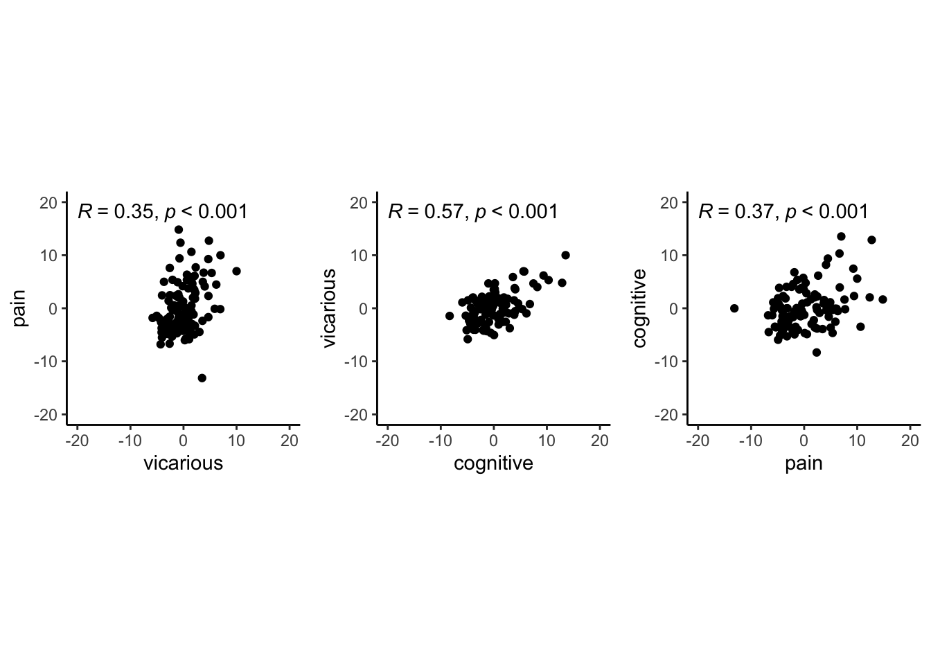

ggsave(save_plotname, width = 10, height = 3)

6.2.5 model 04 4-4 lineplot

library(ggpubr)
DATA = as.data.frame(combined_se_calc_cooksd)
color = c( "#4575B4", "#D73027")
LINEIV1 = "stim_ordered"
LINEIV2 = "cue_ordered"
MEAN = "mean_per_sub_norm_mean"
ERROR = "ci"
dv_keyword = "actual"
p1 = plot_lineplot_twofactor(DATA, 'pain', 
               LINEIV1, LINEIV2, MEAN, ERROR, color, ggtitle = 'pain' )
p2 = plot_lineplot_twofactor(DATA,'vicarious', 
               LINEIV1, LINEIV2, MEAN, ERROR, color,ggtitle = 'vicarious')
p3 = plot_lineplot_twofactor(DATA, 'cognitive', 
               LINEIV1, LINEIV2, MEAN, ERROR, color,ggtitle = 'cognitive')
#grid.arrange(p1, p2, p3, ncol=3 , common.legend = TRUE)
ggpubr::ggarrange(p1,p2,p3,ncol = 3, nrow = 1, common.legend = TRUE,legend = "bottom")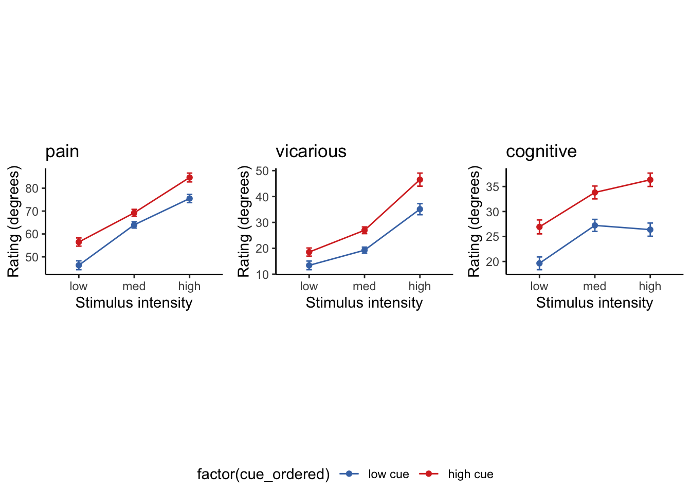

plot_filename = file.path(analysis_dir,
                          paste('lineplot_task-all_rating-',dv_keyword,'.png', sep = ""))
ggsave(plot_filename, width = 8, height = 4)