Chapter 7 [beh] RT ~ cue
What is the purpose of this notebook?
Here, I test the cue effect (high vs. low) on Reaction time and performance in the cogntive, mental-rotation tasks
- left = diff, right = same
- model 1: Does RT differ as a function of cue type?
- model 1-1: Does RT differ as a function of cue, ONLY for the correct trials?
- model 1-2: Does RT differ as a function of cue, ONLY for the incorrect trials?
- model 2: would log-transforming help? Do we see a cue effect on the log-transformmed RTs?
7.0.2 1) plot RT data
# parameters _____________________________________ # nolint
subject_varkey <- "src_subject_id"
iv <- "param_cue_type"
dv <- "event03_RT"
dv_keyword <- "RT"
xlab <- ""
taskname <- "cognitive"
ylab <- "ratings (degree)"
subject <- "subject"
exclude <- "sub-0999|sub-0001|sub-0002|sub-0003|sub-0004|sub-0005|sub-0006|sub-0007|sub-0008|sub-0009|sub-0010|sub-0011"

data <- load_task_social_df(datadir, taskname = taskname, subject_varkey = subject_varkey, iv = iv,  exclude = exclude)
data$event03_RT <- data$event03_stimulusC_reseponseonset - data$event03_stimulus_displayonset
7.0.3 plot RT distribution per participant
- the purpose is to identify whether RTs are distributed from 0-5 sec or not
ggplot(data,aes(x=event03_RT, group = subject)) +
  geom_histogram(color="darkblue", fill="lightblue", binwidth=0.25, bins = 20) +
  facet_wrap(~subject, ncol = 10) +
  theme(axis.text=element_text(size=5),text=element_text(size=6))
## Warning: Removed 591 rows containing non-finite values (`stat_bin()`).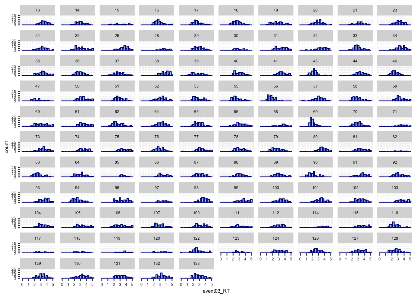
- some participants may not have responded within time limit
- the button may not have registered the correct onset
- I may have to remove the RTs with 5 sec.
7.0.4 exclude participants with RT of 5 seconds
# parameters _____________________________________ # nolint
subject_varkey <- "src_subject_id"
iv <- "param_cue_type"
dv <- "event03_RT"
dv_keyword <- "RT"
xlab <- ""
taskname <- "cognitive"

ylab <- "ratings (degree)"
subject <- "subject"
exclude <- "sub-0999|sub-0001|sub-0002|sub-0003|sub-0004|sub-0005|sub-0006|sub-0007|sub-0008|sub-0009|sub-0010|sub-0011"

# load data _____________________________________
data <- load_task_social_df(datadir, taskname = taskname, subject_varkey = subject_varkey, iv = iv, exclude = exclude)
data$event03_RT <- data$event03_stimulusC_reseponseonset - data$event03_stimulus_displayonset

analysis_dir <- file.path(main_dir, "analysis", "mixedeffect", "model05_iv-cue_dv-RT", as.character(Sys.Date()))
dir.create(analysis_dir, showWarnings = FALSE, recursive = TRUE)

data$event03_response_samediff <- mapvalues(data$event03_stimulusC_response,
                                                from = c(1, 2),
                                                to = c("diff", "same"))

data$event03_correct <- ifelse(data$event03_C_stim_match == data$event03_response_samediff, 1, ifelse(data$event03_C_stim_match != data$event03_response_samediff, 0, "NA"))
7.1 model 1:
- plotting all of the code
- Does RT differ as a function of high vs. low cue?
- conclusion: No. RT does not differ as a function of cue
# parameters ________________________________
subject_varkey <- "src_subject_id"
iv <- "param_cue_type"
dv <- "event03_RT"
dv_keyword <- "RT"
xlab <- ""
taskname <- "cognitive"
ylim = c(0,5)

# lmer filename ________________________________
model_savefname <- file.path(
        analysis_dir,
        paste("lmer_task-", taskname,
            "_rating-", dv_keyword,
            "_", as.character(Sys.Date()), ".txt",
            sep = ""
        )
    )

# removing NA values ________________________________
data_clean = data[!is.na(data$event03_correct),]
data_clean$subject = factor(data_clean$src_subject_id)

# lmer model ________________________________
sink(model_savefname)
model_onefactor <- lmer(event03_RT ~ param_cue_type + (1 | subject), data = data_clean)
summary(model_onefactor)
## Linear mixed model fit by REML. t-tests use Satterthwaite's method [
## lmerModLmerTest]
## Formula: event03_RT ~ param_cue_type + (1 | subject)
## Data: data_clean
##
## REML criterion at convergence: 14209.8
##
## Scaled residuals:
## Min 1Q Median 3Q Max
## -4.6862 -0.7107 -0.0840 0.6761 3.4733
##
## Random effects:
## Groups Name Variance Std.Dev.
## subject (Intercept) 0.1642 0.4052
## Residual 0.5533 0.7439
## Number of obs: 6189, groups: subject, 105
##
## Fixed effects:
## Estimate Std. Error df t value Pr(>|t|)
## (Intercept) 3.16779 0.04193 115.61558 75.552 <2e-16 ***
## param_cue_typelow_cue -0.03041 0.01892 6084.64140 -1.607 0.108
## ---
## Signif. codes: 0 '***' 0.001 '**' 0.01 '*' 0.05 '.' 0.1 ' ' 1
##
## Correlation of Fixed Effects:
## (Intr)
## prm_c_typl_ -0.225sink()
fixEffect <- as.data.frame(fixef(model_onefactor))
randEffect <- as.data.frame(ranef(model_onefactor))
cooksd <- cooks.distance(model_onefactor)
influential <- as.numeric(names(cooksd)[
(cooksd > (4 / as.numeric(length(unique(data_clean$subject)))))])
data_screen <- data_clean[-influential, ]
# summary statistics for plots ________________________________
subjectwise <- meanSummary(data_screen, c(subject, iv), dv)
groupwise <- summarySEwithin(
data = subjectwise,
measurevar = "mean_per_sub", # variable created from above
withinvars = c(iv), # iv
idvar = "subject"
)##
## Attaching package: 'raincloudplots'## The following object is masked _by_ '.GlobalEnv':
##
## GeomFlatViolin## Automatically converting the following non-factors to factors: param_cue_typesubjectwise_mean <- "mean_per_sub"; group_mean <- "mean_per_sub_norm_mean"
se <- "se"; subject <- "subject"
ggtitle <- paste(taskname, " - Reaction Time (s)"); title <- paste(taskname, " - RT")
xlab <- ""; ylab <- "Reaction Time (s)";
w = 5; h = 3; dv_keyword <- "RT"
if (any(startsWith(dv_keyword, c("expect", "Expect")))) {
color <- c("#1B9E77", "#D95F02")
} else {
color <- c("#4575B4", "#D73027")
}
plot_savefname <- file.path(
analysis_dir,
paste("raincloud_task-", taskname,
"_dv-", dv_keyword,
"_", as.character(Sys.Date()), ".png",
sep = ""
)
)
plot_halfrainclouds_onefactor(
subjectwise, groupwise,
iv, subjectwise_mean, group_mean, se, subject,
ggtitle, title, xlab, ylab, task_name, ylim,
w, h, dv_keyword, color, plot_savefname
)## Warning in geom_line(data = subjectwise, aes(group = .data[[subject]], x =
## as.numeric(as.factor(.data[[iv]])) - : Ignoring unknown aesthetics: fill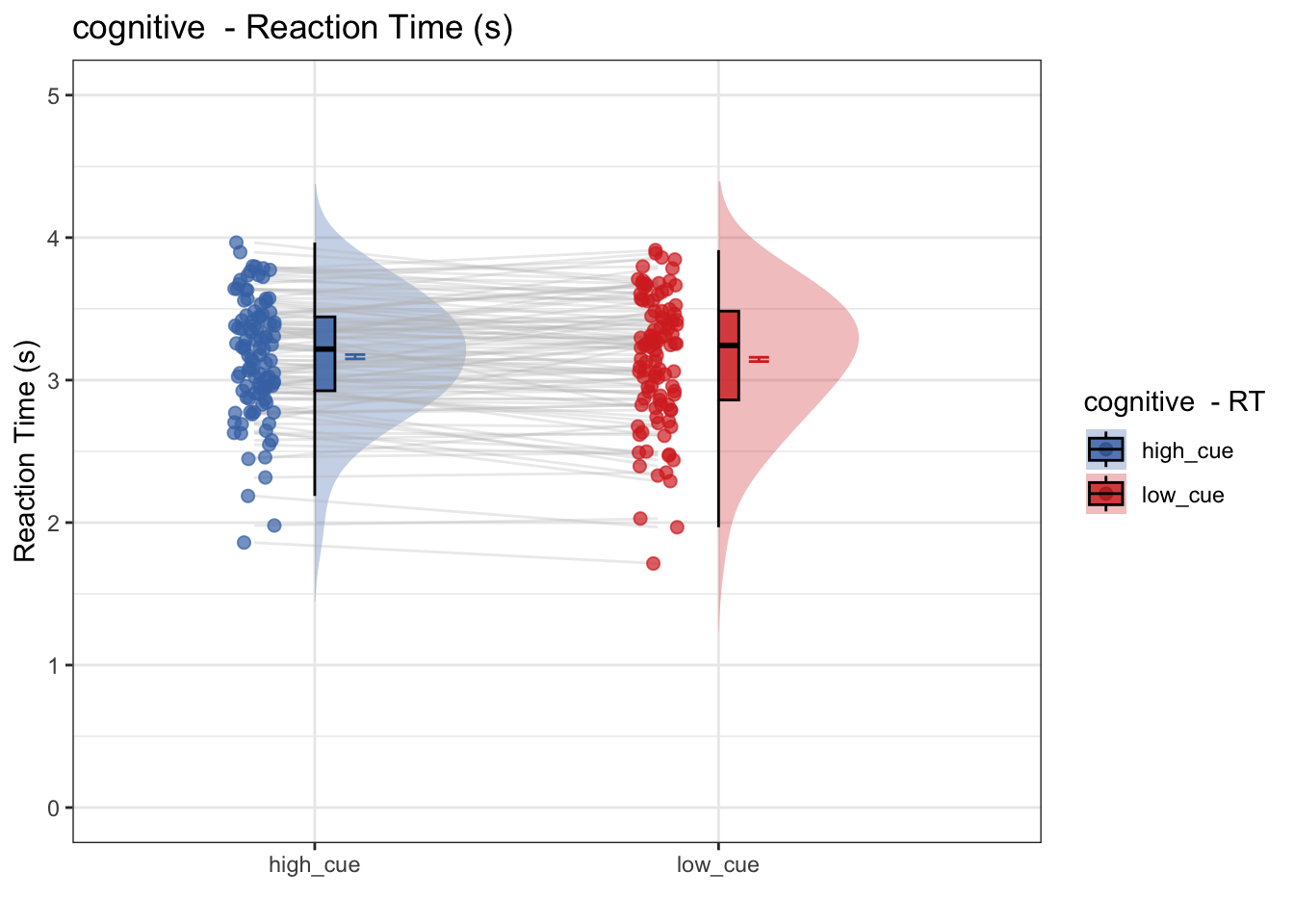
# random effects ________________________________
randEffect <- as.data.frame(ranef(model_onefactor))
fixEffect <- as.data.frame(fixef(model_onefactor))
randEffect$newcoef <- mapvalues(randEffect$term,
    from = c("(Intercept)",
             "param_cue_typelow_cue"
             ),
    to = c("rand_intercept", "rand_cue")
)
## The following `from` values were not present in `x`: param_cue_typelow_cuerand_subset <- subset(randEffect, select = -c(grpvar, term, condsd))
wide_rand <- spread(rand_subset, key = newcoef, value = condval)
wide_fix <- do.call(
"rbind",
replicate(nrow(wide_rand),
as.data.frame(t(as.matrix(fixEffect))),
simplify = FALSE
)
)
rownames(wide_fix) <- NULL
new_wide_fix <- dplyr::rename(wide_fix,
fix_intercept = `(Intercept)`,
fix_cue = `param_cue_typelow_cue`,
)
total <- cbind(wide_rand, new_wide_fix)
total$task <- taskname
new_total <- total %>% dplyr::select(task, everything())
new_total <- dplyr::rename(total, subj = grp)
rand_savefname <- file.path(
analysis_dir,
paste("randeffect_task-", taskname, "_",
as.character(Sys.Date()), "_outlier-cooksd.csv",
sep = ""
)
)
write.csv(new_total, rand_savefname, row.names = FALSE)7.2 model 1-1
- omitting code (identical to model 1, except for subsetting correct trials)
- Only using correct trials, does RT differ as a function of high vs. low cue?
- conclusion 1-1: No. Even within the subset of correct trials, RT does not differ as a function of cue
## Linear mixed model fit by REML. t-tests use Satterthwaite's method [
## lmerModLmerTest]
## Formula: event03_RT ~ param_cue_type + (1 | subject)
##    Data: data_c
##
## REML criterion at convergence: 11663.2
##
## Scaled residuals:
##     Min      1Q  Median      3Q     Max
## -4.7110 -0.7072 -0.0918  0.6810  3.5074
##
## Random effects:
##  Groups   Name        Variance Std.Dev.
##  subject  (Intercept) 0.1665   0.4080
##  Residual             0.5528   0.7435
## Number of obs: 5066, groups:  subject, 105
##
## Fixed effects:
##                         Estimate Std. Error         df t value Pr(>|t|)
## (Intercept)              3.15735    0.04278  118.28326  73.803   <2e-16 ***
## param_cue_typelow_cue   -0.02213    0.02094 4965.87720  -1.057    0.291
## ---
## Signif. codes:  0 '***' 0.001 '**' 0.01 '*' 0.05 '.' 0.1 ' ' 1
##
## Correlation of Fixed Effects:
##             (Intr)
## prm_c_typl_ -0.245
## Automatically converting the following non-factors to factors: param_cue_type## Warning in geom_line(data = subjectwise, aes(group = .data[[subject]], x =
## as.numeric(as.factor(.data[[iv]])) - : Ignoring unknown aesthetics: fill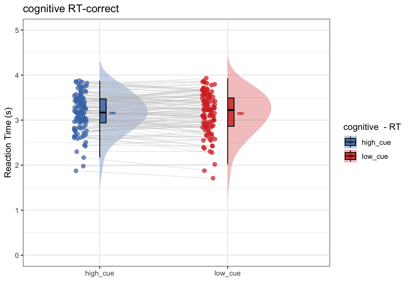
## The following `from` values were not present in `x`: param_cue_typelow_cue7.3 model 1-2:
- omitting code (identical to model 1, except for subsetting incorrect trials)
- Only using incorrect trials, does RT differ as a function of high vs. low cue?
- conclusion 1-2: no. Even within the subset of incorrect trials, RT does not differ as a function of cue
## Linear mixed model fit by REML. t-tests use Satterthwaite's method [
## lmerModLmerTest]
## Formula: event03_RT ~ param_cue_type + (1 | subject)
##    Data: data_i
##
## REML criterion at convergence: 2668
##
## Scaled residuals:
##     Min      1Q  Median      3Q     Max
## -4.1263 -0.7154 -0.0559  0.6479  2.8124
##
## Random effects:
##  Groups   Name        Variance Std.Dev.
##  subject  (Intercept) 0.1518   0.3897
##  Residual             0.5564   0.7459
## Number of obs: 1123, groups:  subject, 103
##
## Fixed effects:
##                         Estimate Std. Error         df t value Pr(>|t|)
## (Intercept)              3.19726    0.05117  146.23721  62.480   <2e-16 ***
## param_cue_typelow_cue   -0.07195    0.04574 1065.34392  -1.573    0.116
## ---
## Signif. codes:  0 '***' 0.001 '**' 0.01 '*' 0.05 '.' 0.1 ' ' 1
##
## Correlation of Fixed Effects:
##             (Intr)
## prm_c_typl_ -0.438
## Automatically converting the following non-factors to factors: param_cue_type## Warning in geom_line(data = subjectwise, aes(group = .data[[subject]], x =
## as.numeric(as.factor(.data[[iv]])) - : Ignoring unknown aesthetics: fill## Warning: Removed 1 rows containing non-finite values (`stat_half_ydensity()`).## Warning: Removed 1 rows containing non-finite values (`stat_boxplot()`).## Warning: Removed 1 row containing missing values (`geom_line()`).## Warning: Removed 1 rows containing missing values (`geom_point()`).## Warning: Removed 1 rows containing non-finite values (`stat_half_ydensity()`).## Warning: Removed 1 rows containing non-finite values (`stat_boxplot()`).## Warning: Removed 1 row containing missing values (`geom_line()`).## Warning: Removed 1 rows containing missing values (`geom_point()`).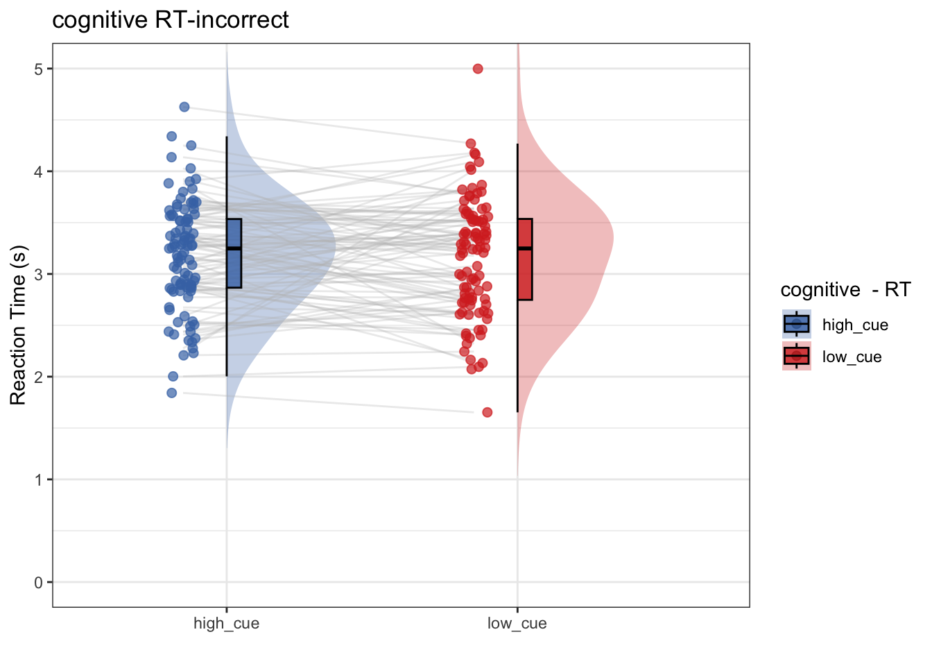
## The following `from` values were not present in `x`: param_cue_typelow_cue7.4 model 2:
- omitting code (identical to model 1, except for log-transformming RT)
- Does log transformming help? After log-transformming RT, does RT differ as a function of high vs. low cue?
- conclusion 2: No, log transformmed or not, there is no significant cue effect on RT
## Linear mixed model fit by REML. t-tests use Satterthwaite's method [
## lmerModLmerTest]
## Formula: log_RT ~ param_cue_type + (1 | subject)
##    Data: data_clean
##
## REML criterion at convergence: 1757.4
##
## Scaled residuals:
##      Min       1Q   Median       3Q      Max
## -23.2005  -0.5846   0.0388   0.6555   2.8309
##
## Random effects:
##  Groups   Name        Variance Std.Dev.
##  subject  (Intercept) 0.02072  0.1439
##  Residual             0.07401  0.2720
## Number of obs: 6189, groups:  subject, 105
##
## Fixed effects:
##                         Estimate Std. Error         df t value Pr(>|t|)
## (Intercept)              1.11345    0.01494  116.68888  74.519   <2e-16 ***
## param_cue_typelow_cue   -0.01130    0.00692 6085.09207  -1.633    0.103
## ---
## Signif. codes:  0 '***' 0.001 '**' 0.01 '*' 0.05 '.' 0.1 ' ' 1
##
## Correlation of Fixed Effects:
##             (Intr)
## prm_c_typl_ -0.231
## Automatically converting the following non-factors to factors: param_cue_type## Warning in geom_line(data = subjectwise, aes(group = .data[[subject]], x =
## as.numeric(as.factor(.data[[iv]])) - : Ignoring unknown aesthetics: fill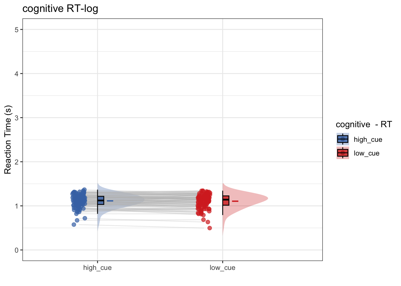
## The following `from` values were not present in `x`: param_cue_typelow_cue