8 beh :: rating variability
Those with greater variability have greater placebo effects.
- Harris (2005) Effect of variability in the 7-day baseline pain diary on the assay sensitivity of neuropathic pain randomized clinical trials: An ACTTION study. doi: 10.1002/art.21407
- Farrar et al (2014) Effect of variability in the 7-day baseline pain diary on the assay sensitivity of neuropathic pain randomized clinical trials: An ACTTION study
load libraries
# parameters ___________________________________________________________________
main_dir <- dirname(dirname(getwd()))
datadir <- file.path(main_dir, 'data', 'beh', 'beh02_preproc')
analysis_dir <- file.path(main_dir, "analysis", "mixedeffect", "model09_var", as.character(Sys.Date()))
dir.create(analysis_dir, showWarnings = FALSE, recursive = TRUE)
subject_varkey <- "src_subject_id"
iv <- "param_cue_type"
dv <- "event03_RT"
dv_keyword <- "RT"
xlab <- ""
taskname <- "pain"
ylab <- "ratings (degree)"
subject <- "subject"
exclude <- "sub-0001"
# 1. load data _________________________________________________________________
data <- cueR::df_load_beh(datadir,
                            taskname = taskname,
                            subject_varkey = subject_varkey,
                            iv = iv,
                            exclude = exclude)

column_mapping <- c("src_subject_id" = "subject",
                    "session_id" = "ses",
                    "param_run_num" = "run",
                    "param_task_name" = "runtype",
                    "param_cue_type" = "cue",
                    "param_stimulus_type" = "stimintensity")
data <- df_rename_columns(data, column_mapping)
data_centered <- cueR::compute_enderstofighi(data, sub="subject",
                                    outcome = "event04_actual_angle",expect= "event02_expect_angle",
                                    ses = "ses", run = "run")
8.1 Analysis 1: Pain display distribution of data
Let’s look at the distribution of the data. X axis: Y axis:
# remove NA values first
df.centered_NA <- data_centered %>% filter(!is.na(OUTCOME))  # Remove NA values
head(df.centered_NA)
## # A tibble: 6 × 75
## src_subject_id session_id param_task_name param_run_num param_counterbalance…¹
## <int> <int> <chr> <int> <int>
## 1 2 1 pain 1 3
## 2 2 1 pain 1 3
## 3 2 1 pain 1 3
## 4 2 1 pain 1 3
## 5 2 1 pain 1 3
## 6 2 1 pain 1 3
## # ℹ abbreviated name: ¹param_counterbalance_ver
## # ℹ 70 more variables: param_counterbalance_block_num <int>,
## # param_cue_type <chr>, param_stimulus_type <chr>, param_cond_type <int>,
## # param_trigger_onset <dbl>, param_start_biopac <dbl>, ITI_onset <dbl>,
## # ITI_biopac <dbl>, ITI_duration <dbl>, event01_cue_onset <dbl>,
## # event01_cue_biopac <dbl>, event01_cue_type <chr>,
## # event01_cue_filename <chr>, ISI01_onset <dbl>, ISI01_biopac <dbl>, …8.1.1 Sort based on Median Outcome rating order
# Sort the data by median "outcome" in ascending order
sorted_data <- df.centered_NA %>%
  group_by(subject) %>%
  summarize(median_outcome = median(OUTCOME, na.rm = TRUE)) %>%
  arrange(median_outcome) %>%
  select(subject)

# Reorder the "subject" factor based on the sorted order
df.centered_NA$subject <- factor(df.centered_NA$subject, levels = sorted_data$subject)

# Create the ggplot
g <- ggplot(df.centered_NA, aes(x = subject, y = OUTCOME, fill = subject)) +
  geom_boxplot(outlier.shape = NA, width = 1.2, position = position_dodge(2)) +
  geom_jitter(width = .1, alpha = 0, size = 1) +
  labs(x = "Subject", y = "Pain Outcome Rating") +
  theme_classic() +
  theme(legend.position = "none") +
  scale_x_discrete(breaks = NULL)

# Convert ggplot object to a plotly object with hover information
g_plotly <- ggplotly(ggplot_largetext(g), tooltip = c("x", "y"))
## Warning: `position_dodge()` requires non-overlapping x intervals## Warning: Aspect ratios aren't yet implemented, but you can manually set a
## suitable height/width
## Warning: Aspect ratios aren't yet implemented, but you can manually set a
## suitable height/width
g_plotly8.3 Q. Do those who use the scale widely show greater cue effects?
df.centered_NA$run_order <- NA
dv <- "OUTCOME"

  # 3. calculate difference scores and summarize _____________________________
df.centered_NA$run_order[df.centered_NA$run > 3] <- "a"
df.centered_NA$run_order[df.centered_NA$run <= 3] <- "b"
sub_diff <- subset(df.centered_NA, select = c(
    "subject", "ses", "run",
    "runtype", "cue",
    "stimintensity", dv
))

# drop NA
sub_diff_NA <- sub_diff %>% filter(!is.na(dv))
subjectwise <- meanSummary(sub_diff_NA, c(
    "subject", "ses", "run",
    "runtype", "cue",
    "stimintensity"), dv)

mean_outcome <- subjectwise[1:(length(subjectwise) - 1)]
wide <- mean_outcome %>%
    tidyr::spread(cue, mean_per_sub)
wide$stim_name <- NA
wide$diff <- wide$high_cue - wide$low_cue
wide$stim_name[wide$stimintensity == "high_stim"] <- "high"
wide$stim_name[wide$stimintensity == "med_stim"] <- "med"
wide$stim_name[wide$stimintensity == "low_stim"] <- "low"
wide$stim_ordered <- factor(wide$stim_name,
    levels = c("low", "med", "high")
)


subjectwise_diff <- meanSummary(wide, c("subject"), "diff")
# subjectwise_diff$stim_ordered <- factor(subjectwise_diff$stim_ordered,
#     levels = c("low", "med", "high")
# )
subjectwise_NA <- subjectwise_diff %>% filter(!is.na(sd))
groupwise_diff <- summarySE(
    data = subjectwise_NA,
    measurevar = "mean_per_sub", # variable created from above
    #withinvars = c("stim_ordered"), # iv
    #idvar = "subject"
)

# per stim _____________________________________________________________________
# subjectwise_diff <- meanSummary(wide, c("subject", "stim_ordered"), "diff")
# subjectwise_diff$stim_ordered <- factor(subjectwise_diff$stim_ordered,
#     levels = c("low", "med", "high")
# )
# subjectwise_NA <- subjectwise_diff %>% filter(!is.na(sd))
# groupwise_diff <- summarySEwithin(
#     data = subjectwise_NA,
#     measurevar = "mean_per_sub", # variable created from above
#     withinvars = c("stim_ordered"), # iv
#     idvar = "subject"
# )
cue.iqr <- df.centered_NA %>%
  group_by(subject, cue) %>%
  summarize(IQR = IQR(OUTCOME, na.rm = TRUE)) %>%
  arrange(IQR)
## `summarise()` has grouped output by 'subject'. You can override using the
## `.groups` argument.
model.iqr <- lmer(IQR ~ cue + (1|subject), data = cue.iqr)
summary(model.iqr)
## Linear mixed model fit by REML. t-tests use Satterthwaite's method [
## lmerModLmerTest]
## Formula: IQR ~ cue + (1 | subject)
## Data: cue.iqr
##
## REML criterion at convergence: 1794.4
##
## Scaled residuals:
## Min 1Q Median 3Q Max
## -2.0326 -0.5190 -0.1210 0.4566 2.6943
##
## Random effects:
## Groups Name Variance Std.Dev.
## subject (Intercept) 165.60 12.87
## Residual 66.75 8.17
## Number of obs: 227, groups: subject, 114
##
## Fixed effects:
## Estimate Std. Error df t value Pr(>|t|)
## (Intercept) 29.550 1.431 149.757 20.654 <2e-16 ***
## cuelow_cue 0.831 1.086 111.517 0.765 0.446
## ---
## Signif. codes: 0 '***' 0.001 '**' 0.01 '*' 0.05 '.' 0.1 ' ' 1
##
## Correlation of Fixed Effects:
## (Intr)
## cuelow_cue -0.382our design is conflated with variability and the placebo effect, because the high cues have more variability. but actually no! IQR does not differ as a function of cue leve. There’s more to it!
expect.iqr <- df.centered_NA %>%
  group_by(subject) %>%
  summarize(IQR = IQR(EXPECT, na.rm = TRUE)) %>%
  arrange(IQR)

colnames(expect.iqr)
## [1] "subject" "IQR"
colnames(subjectwise_NA)## [1] "subject" "mean_per_sub" "sd"## subject mean_per_sub sd IQR
## 1 10 10.267275 14.728124 45.927555
## 2 100 5.513644 10.175649 23.331188
## 3 101 8.155616 21.706200 38.016011
## 4 103 -4.610429 9.444593 9.118222
## 5 104 6.278523 18.905402 36.252133
## 6 105 4.393742 13.162857 24.395731
range(merge_cueeffect_IQR$mean_per_sub)## [1] -35.99724 37.83760
range(merge_cueeffect_IQR$IQR)## [1] 6.940743 109.358498
g<- cueR::plot_ggplot_correlation(data = merge_cueeffect_IQR,
                              x = 'mean_per_sub', y = 'IQR',
                                    p_acc = 0.001, r_acc = 0.01,
                                    limit_min = -40, limit_max = 200, label_position = .6)
g + xlab("cue effect (high vs. low cue OUTCOME)") + ylab("EXPECT IQR") + ylim(0,150) + xlim(-50, 50)
## Scale for y is already present.
## Adding another scale for y, which will replace the existing scale.
## Scale for x is already present.
## Adding another scale for x, which will replace the existing scale.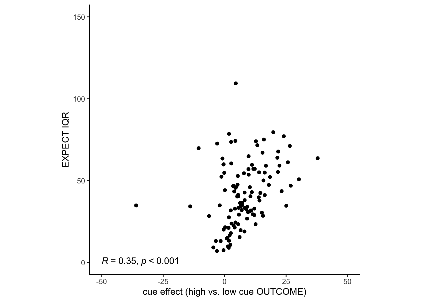
pretty obvious now that i think about it. those with larger cue effects wil have larger IQRs. in order for one to have a cue effect, you do need to report your outcome ratings drastically different depending on the cue presented.
8.4 Here I plot the expectation rating distribution, BUT sorted based on one’s cue effect difference
## subject mean_per_sub sd src_subject_id session_id param_task_name
## 1 10 10.26727 14.72812 10 4 pain
## 2 10 10.26727 14.72812 10 1 pain
## 3 10 10.26727 14.72812 10 3 pain
## 4 10 10.26727 14.72812 10 4 pain
## 5 10 10.26727 14.72812 10 4 pain
## 6 10 10.26727 14.72812 10 4 pain
## param_run_num param_counterbalance_ver param_counterbalance_block_num
## 1 2 4 2
## 2 6 4 1
## 3 3 4 1
## 4 2 4 2
## 5 2 4 2
## 6 2 4 2
## param_cue_type param_stimulus_type param_cond_type param_trigger_onset
## 1 low_cue med_stim 2 1616614186
## 2 low_cue low_stim 1 1615231970
## 3 high_cue high_stim 6 1616008227
## 4 low_cue med_stim 2 1616614186
## 5 high_cue low_stim 4 1616614186
## 6 high_cue low_stim 4 1616614186
## param_start_biopac ITI_onset ITI_biopac ITI_duration event01_cue_onset
## 1 1616614186 1616614549 1616614549 3.5644388 1616614553
## 2 1615231970 1615232215 1615232215 0.6961169 1615232216
## 3 1616008227 1616008469 1616008469 2.1638486 1616008471
## 4 1616614186 1616614225 1616614225 0.9021652 1616614226
## 5 1616614186 1616614480 1616614480 3.8734350 1616614484
## 6 1616614186 1616614521 1616614521 0.8413310 1616614522
## event01_cue_biopac event01_cue_type event01_cue_filename ISI01_onset
## 1 1616614553 low_cue l007.png 1616614554
## 2 1615232216 low_cue l039.png 1615232217
## 3 1616008471 high_cue h003.png 1616008472
## 4 1616614226 low_cue l003.png 1616614227
## 5 1616614484 high_cue h028.png 1616614485
## 6 1616614522 high_cue h009.png 1616614523
## ISI01_biopac ISI01_duration event02_expect_displayonset event02_expect_biopac
## 1 1616614554 0.8951526 1616614555 1616614555
## 2 1615232217 2.0953798 1615232219 1615232219
## 3 1616008472 1.9952071 1616008474 1616008474
## 4 1616614227 1.9835362 1616614229 1616614229
## 5 1616614485 1.7873995 1616614487 1616614487
## 6 1616614523 1.8900447 1616614525 1616614525
## event02_expect_responseonset event02_expect_RT event02_expect_angle
## 1 1616614556 1.617795 2.070031
## 2 1615232220 1.518819 36.869898
## 3 1616008477 3.368093 55.799516
## 4 1616614232 3.089105 40.451958
## 5 1616614490 2.976417 99.462322
## 6 1616614527 2.601101 71.417000
## event02_expect_angle_label ISI02_onset ISI02_biopac ISI02_duration
## 1 FIX 1616614559 1616614559 7.5599790
## 2 FIX 1615232223 1615232223 4.5597293
## 3 FIX 1616008478 1616008478 0.6596248
## 4 FIX 1616614233 1616614233 0.5646281
## 5 FIX 1616614491 1616614491 14.6685627
## 6 FIX 1616614529 1616614529 0.7711728
## event03_stimulus_type event03_stimulus_displayonset event03_stimulus_biopac
## 1 med_stim 1616614566 1616614566
## 2 low_stim 1615232228 1615232228
## 3 high_stim 1616008479 1616008479
## 4 med_stim 1616614234 1616614234
## 5 low_stim 1616614506 1616614506
## 6 low_stim 1616614529 1616614529
## event03_stimulus_C_stim_match event03_stimulusC_response
## 1 NA 0
## 2 NA 0
## 3 NA 0
## 4 NA 0
## 5 NA 0
## 6 NA 0
## event03_stimulusC_responsekeyname event03_stimulusC_reseponseonset
## 1 NA 0
## 2 NA 0
## 3 NA 0
## 4 NA 0
## 5 NA 0
## 6 NA 0
## event03_stimulusC_RT ISI03_onset ISI03_biopac ISI03_duration
## 1 0 1616614575 1616614575 4.987133
## 2 0 1615232237 1615232237 4.287938
## 3 0 1616008488 1616008488 1.989352
## 4 0 1616614243 1616614243 6.494392
## 5 0 1616614515 1616614515 2.193067
## 6 0 1616614538 1616614538 6.684188
## event04_actual_displayonset event04_actual_biopac
## 1 1616614580 1616614580
## 2 1615232241 1615232241
## 3 1616008490 1616008490
## 4 1616614249 1616614249
## 5 1616614517 1616614517
## 6 1616614545 1616614545
## event04_actual_responseonset event04_actual_RT event04_actual_angle
## 1 1616614583 2.508353 33.562744
## 2 1615232244 2.684495 13.253716
## 3 1616008493 3.525335 69.957683
## 4 1616614252 2.417763 28.316355
## 5 1616614519 1.984204 9.954607
## 6 1616614548 2.704694 20.609693
## event04_actual_angle_label param_end_instruct_onset param_end_biopac
## 1 FIX 1616614584 1616614584
## 2 FIX 1615232368 1615232368
## 3 FIX 1616008626 1616008626
## 4 FIX 1616614584 1616614584
## 5 FIX 1616614584 1616614584
## 6 FIX 1616614584 1616614584
## param_experiment_duration event03_stimulus_P_trigger
## 1 398.5102 Command Recieved: TRIGGER_AND_Response: RESULT_OK
## 2 398.1037 Command Recieved: TRIGGER_AND_Response: RESULT_OK
## 3 399.0270 Command Recieved: TRIGGER_AND_Response: RESULT_OK
## 4 398.5102 Command Recieved: TRIGGER_AND_Response: RESULT_OK
## 5 398.5102 Command Recieved: TRIGGER_AND_Response: RESULT_OK
## 6 398.5102 Command Recieved: TRIGGER_AND_Response: RESULT_OK
## event03_stimulus_P_delay_between_medoc event03_stimulus_V_patientid
## 1 0 NA
## 2 0 NA
## 3 0 NA
## 4 0 NA
## 5 0 NA
## 6 0 NA
## event03_stimulus_V_filename event03_stimulus_C_stim_num
## 1 NA 0
## 2 NA 0
## 3 NA 0
## 4 NA 0
## 5 NA 0
## 6 NA 0
## event03_stimulus_C_stim_filename delay_between_medoc ses run runtype cue
## 1 NA 0.05064011 4 2 pain low_cue
## 2 NA 0.05586195 1 6 pain low_cue
## 3 NA 0.04395199 3 3 pain high_cue
## 4 NA 0.08373189 4 2 pain low_cue
## 5 NA 0.06575012 4 2 pain high_cue
## 6 NA 0.04667401 4 2 pain high_cue
## stimintensity OUTCOME EXPECT OUTCOME_cm OUTCOME_demean EXPECT_cm
## 1 med_stim 33.562744 2.070031 40.66489 -7.102146 42.56259
## 2 low_stim 13.253716 36.869898 40.66489 -27.411174 42.56259
## 3 high_stim 69.957683 55.799516 40.66489 29.292793 42.56259
## 4 med_stim 28.316355 40.451958 40.66489 -12.348535 42.56259
## 5 low_stim 9.954607 99.462322 40.66489 -30.710283 42.56259
## 6 low_stim 20.609693 71.417000 40.66489 -20.055197 42.56259
## EXPECT_demean OUTCOME_zscore EXPECT_zscore trial_index lag.OUTCOME_demean
## 1 -40.492556 -0.3268431 -1.40964500 12 -20.05520
## 2 -5.692689 -1.2614711 -0.19817644 9 43.30186
## 3 13.236929 1.3480638 0.46080992 8 -19.97422
## 4 -2.110629 -0.5682836 -0.07347616 2 -28.36097
## 5 56.899736 -1.4132971 1.98081910 10 46.57600
## 6 28.854414 -0.9229466 1.00449278 11 -30.71028
## EXPECT_cmc OUTCOME_cmc run_order
## 1 -18.68492 -23.95299 b
## 2 -18.68492 -23.95299 a
## 3 -18.68492 -23.95299 b
## 4 -18.68492 -23.95299 b
## 5 -18.68492 -23.95299 b
## 6 -18.68492 -23.95299 b
# validate _____________________________________________________________________
# sorted_data <- merge_df_cue %>%
#   group_by(subject) %>%
#   arrange(mean_per_sub)

# Reorder the "subject" factor based on the sorted order
g <- ggplot(merge_df_cue, aes(x = reorder(subject, mean_per_sub), y = EXPECT, fill = subject)) +
  geom_boxplot(outlier.shape = NA, width = 1.2, position = position_dodge(2)) +
  geom_jitter(width = .1, alpha = 0, size = 1) +
  labs(x = "Subject (sorted based on Cue effect size (High vs. Low Outcome rating)", y = "Pain Expect Rating") +
  theme_classic() +
  theme(legend.position = "none") +
  scale_x_discrete(breaks = NULL)

# Convert ggplot object to a plotly object with hover information
g_plotly <- ggplotly(ggplot_largetext(g), tooltip = c("x", "y"))
## Warning: `position_dodge()` requires non-overlapping x intervals## Warning: Aspect ratios aren't yet implemented, but you can manually set a
## suitable height/width
## Warning: Aspect ratios aren't yet implemented, but you can manually set a
## suitable height/width
g_plotly8.5 those who use the scale widely will have greater cue effects, simply because they use the scale widely!
But that doesn’t necessarily indicate that their expectation and cue correlations should be high Those with grater scale use, also susceiptible to cues? wider IQR -> greater correlation with expectation and outcome ratings? > The more wider the scale you use, the more likely your expectation and outcome ratings are corerlated this makes sense, because if you have anchoring bias, your expectation will follow the cue, and thereby the scale might be wider? compared to those who ignore the cue? I’m not sure.
# expect.iqr <- df.centered_NA %>%
#   group_by(subject) %>%
#   summarize(IQR = IQR(EXPECT, na.rm = TRUE)) %>%
#   arrange(IQR)
head(df.centered_NA)
## # A tibble: 6 × 76
## src_subject_id session_id param_task_name param_run_num param_counterbalance…¹
## <int> <int> <chr> <int> <int>
## 1 2 1 pain 1 3
## 2 2 1 pain 1 3
## 3 2 1 pain 1 3
## 4 2 1 pain 1 3
## 5 2 1 pain 1 3
## 6 2 1 pain 1 3
## # ℹ abbreviated name: ¹param_counterbalance_ver
## # ℹ 71 more variables: param_counterbalance_block_num <int>,
## # param_cue_type <chr>, param_stimulus_type <chr>, param_cond_type <int>,
## # param_trigger_onset <dbl>, param_start_biopac <dbl>, ITI_onset <dbl>,
## # ITI_biopac <dbl>, ITI_duration <dbl>, event01_cue_onset <dbl>,
## # event01_cue_biopac <dbl>, event01_cue_type <chr>,
## # event01_cue_filename <chr>, ISI01_onset <dbl>, ISI01_biopac <dbl>, …
corr_n_iqr <- df.centered_NA %>%
  dplyr::group_by(subject) %>%
  dplyr::summarise(
    correlation = cor(EXPECT, OUTCOME, use = "complete.obs"),
    IQR = IQR(EXPECT, na.rm = TRUE)
  )

ggplot(corr_n_iqr, aes(x = correlation, y = IQR)) +
  geom_point() +  # This adds the scatter plot points
  theme_classic() +  # Optional: Adds a minimal theme to the plot
  # coord_fixed(aspect.ratio = 1) +
  labs(
    title = "Scatter Plot of Correlation vs. IQR",
    x = "Correlation",
    y = "IQR"
  )
## Warning: Removed 1 rows containing missing values (`geom_point()`).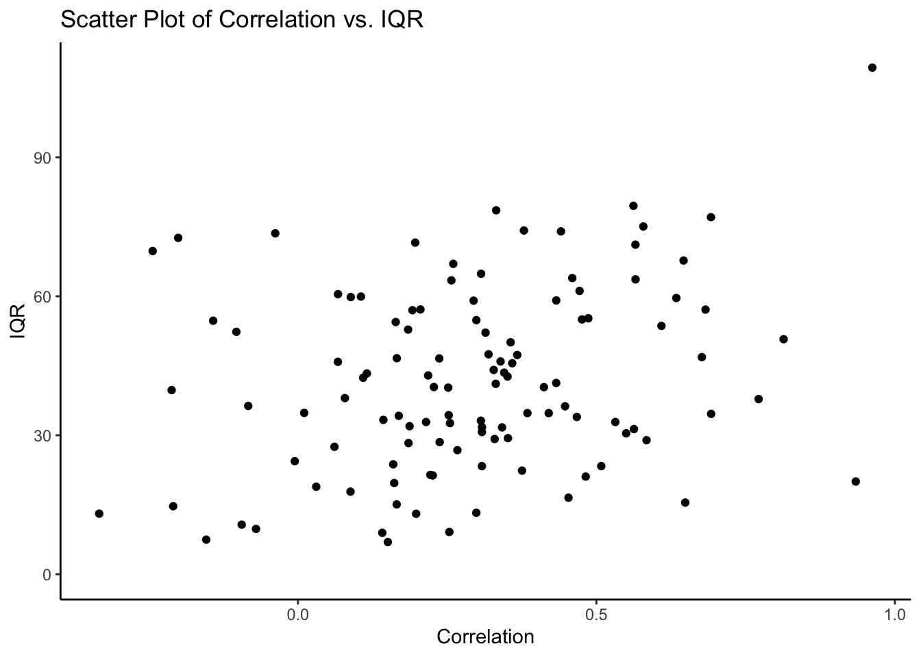
cueR::plot_ggplot_correlation(data = corr_n_iqr, x = 'correlation', y = 'IQR',
                                    p_acc = 0.001, r_acc = 0.01,
                                    limit_min = -40, limit_max = 200, label_position = .6)
## Warning: Removed 1 rows containing non-finite values (`stat_cor()`).
## Removed 1 rows containing missing values (`geom_point()`).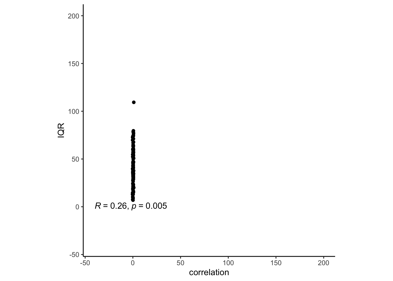
8.5.1 Sort based on IQR
sorted_data <- df.centered_NA %>%
  group_by(subject) %>%
  summarize(IQR = IQR(OUTCOME, na.rm = TRUE)) %>%
  arrange(IQR)
# Reorder the "subject" factor based on the sorted order
df.centered_NA$subject <- factor(df.centered_NA$subject, levels = sorted_data$subject)

# Create the ggplot
g <- ggplot(df.centered_NA, aes(x = subject, y = OUTCOME, fill = subject)) +
  geom_boxplot(outlier.shape = NA, width = 1.2, position = position_dodge(2)) +
  geom_jitter(width = .1, alpha = 0, size = 1) +
  labs(x = "Subject", y = "Pain Outcome Rating") +
  theme_classic() +
  theme(legend.position = "none") +
  scale_x_discrete(breaks = NULL)

# Convert ggplot object to a plotly object with hover information
g_plotly <- ggplotly(ggplot_largetext(g), tooltip = c("x", "y"))
## Warning: `position_dodge()` requires non-overlapping x intervals## Warning: Aspect ratios aren't yet implemented, but you can manually set a
## suitable height/width
## Warning: Aspect ratios aren't yet implemented, but you can manually set a
## suitable height/width
g_plotly