2 beh :: expectation ~ cue
What is the purpose of this notebook?
Here, I plot the expectation ratings as a function of cue.
- Main model:
lmer(expect_rating ~ cue) - Main question: do expectations ratings differ as a function of cue type?
- If there is a main effect of cue on expectation ratings, does this cue effect differ depending on task type?
- IV: cue (high / low)
- DV: expectation rating
Also, Do those who have larger IQRs for expectation ratings also show greater cue effects? Steps: calculate cue effects per pariticpant (high vs. low cue average) calculate IQR per participant check correlation
for (taskname in c("pain", "vicarious", "cognitive")) {
    dv_keyword <- "expect"
    model_savefname <- file.path(
        analysis_dir,
        paste("lmer_task-", taskname,
            "_rating-", dv_keyword,
            "_", as.character(Sys.Date()), ".txt",
            sep = ""
        )
    )
    iv <- "param_stimulus_type"
    dv <- "event02_expect_angle"
    subject_varkey <- "src_subject_id"

    print_lmer_output = TRUE
    exclude <- "sub-0001|sub-0999"
    # load data, run model, and exclude outliers
    data <- df_load_beh(datadir, taskname, subject_varkey, iv, dv, exclude)
    ############################################################################
    # TODO: substitue with cueR::simple_contrast_beh(data)  right before iv <-"stim_ordered"
    data$subject = factor(data$src_subject_id)
    data$stim_name[data$param_stimulus_type == "high_stim"] <- "high"
    data$stim_name[data$param_stimulus_type == "med_stim"] <- "med"
    data$stim_name[data$param_stimulus_type == "low_stim"] <- "low"

    data$stimlin[data$param_stimulus_type == "high_stim"] <- 0.5
    data$stimlin[data$param_stimulus_type == "med_stim"] <- 0
    data$stimlin[data$param_stimulus_type == "low_stim"] <- -0.5

    data$stimquad[data$param_stimulus_type == "high_stim"] <- -0.34
    data$stimquad[data$param_stimulus_type == "med_stim"] <- 0.66
    data$stimquad[data$param_stimulus_type == "low_stim"] <- -0.34

        data$cue_name[data$param_cue_type == "high_cue"] <- "high"
    data$cue_name[data$param_cue_type == "low_cue"] <- "low"

            data$cue_con[data$param_cue_type == "high_cue"] <- 0.5
    data$cue_con[data$param_cue_type == "low_cue"] <- -0.5
    # DATA$levels_ordered <- factor(DATA$param_stimulus_type, levels=c("low", "med", "high"))

    data$stim_ordered <- factor(
        data$stim_name,
        levels = c("low", "med", "high")
    )
    ############################################################################
    iv <- "stim_ordered"
    dv <- "event02_expect_angle"
    print(taskname)
    model <- lmer(event02_expect_angle ~ cue_con + (1|src_subject_id), data = data)
    print(summary(model))
}
## [1] "pain"
## Linear mixed model fit by REML. t-tests use Satterthwaite's method [
## lmerModLmerTest]
## Formula: event02_expect_angle ~ cue_con + (1 | src_subject_id)
## Data: data
##
## REML criterion at convergence: 56012.8
##
## Scaled residuals:
## Min 1Q Median 3Q Max
## -5.1273 -0.6288 -0.0305 0.6197 4.8504
##
## Random effects:
## Groups Name Variance Std.Dev.
## src_subject_id (Intercept) 831.9 28.84
## Residual 529.5 23.01
## Number of obs: 6095, groups: src_subject_id, 114
##
## Fixed effects:
## Estimate Std. Error df t value Pr(>|t|)
## (Intercept) 60.9943 2.7230 113.0814 22.40 <2e-16 ***
## cue_con 34.4542 0.5899 5981.2865 58.41 <2e-16 ***
## ---
## Signif. codes: 0 '***' 0.001 '**' 0.01 '*' 0.05 '.' 0.1 ' ' 1
##
## Correlation of Fixed Effects:
## (Intr)
## cue_con 0.000
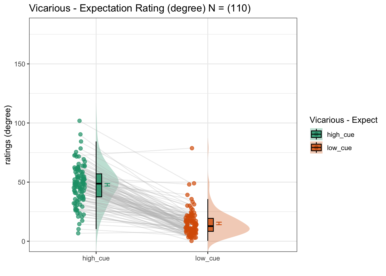
## [1] "vicarious"
## Linear mixed model fit by REML. t-tests use Satterthwaite's method [
## lmerModLmerTest]
## Formula: event02_expect_angle ~ cue_con + (1 | src_subject_id)
## Data: data
##
## REML criterion at convergence: 57065.6
##
## Scaled residuals:
## Min 1Q Median 3Q Max
## -4.3554 -0.6080 -0.0778 0.5620 6.2802
##
## Random effects:
## Groups Name Variance Std.Dev.
## src_subject_id (Intercept) 116.5 10.79
## Residual 293.8 17.14
## Number of obs: 6656, groups: src_subject_id, 114
##
## Fixed effects:
## Estimate Std. Error df t value Pr(>|t|)
## (Intercept) 31.1604 1.0368 112.8038 30.05 <2e-16 ***
## cue_con 33.7887 0.4205 6542.0225 80.36 <2e-16 ***
## ---
## Signif. codes: 0 '***' 0.001 '**' 0.01 '*' 0.05 '.' 0.1 ' ' 1
##
## Correlation of Fixed Effects:
## (Intr)
## cue_con 0.002
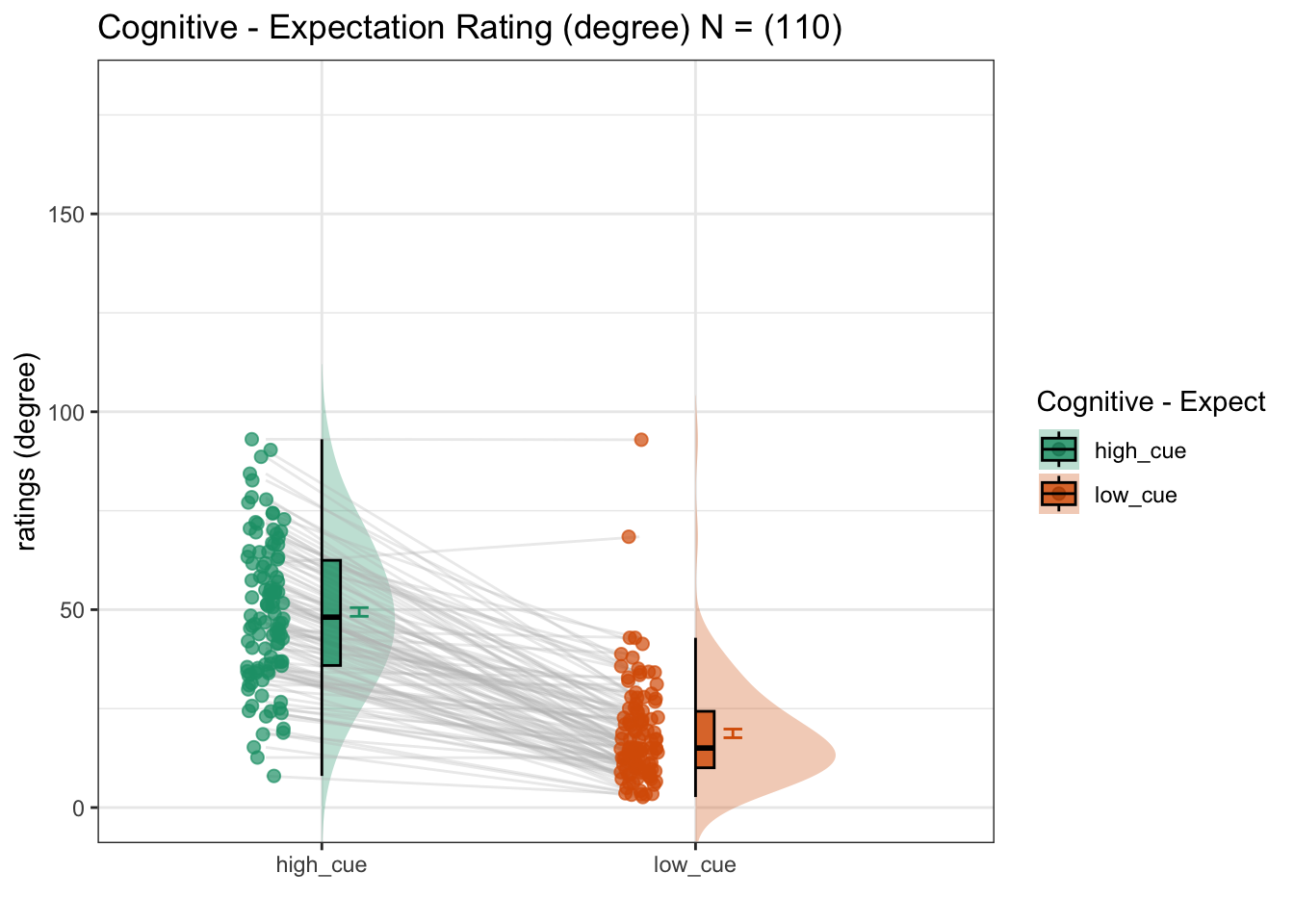
## [1] "cognitive"
## Linear mixed model fit by REML. t-tests use Satterthwaite's method [
## lmerModLmerTest]
## Formula: event02_expect_angle ~ cue_con + (1 | src_subject_id)
## Data: data
##
## REML criterion at convergence: 58008
##
## Scaled residuals:
## Min 1Q Median 3Q Max
## -3.3780 -0.6120 -0.0800 0.5341 9.3354
##
## Random effects:
## Groups Name Variance Std.Dev.
## src_subject_id (Intercept) 167.4 12.94
## Residual 303.3 17.41
## Number of obs: 6737, groups: src_subject_id, 114
##
## Fixed effects:
## Estimate Std. Error df t value Pr(>|t|)
## (Intercept) 33.8866 1.2332 112.1041 27.48 <2e-16 ***
## cue_con 31.7535 0.4246 6622.2852 74.78 <2e-16 ***
## ---
## Signif. codes: 0 '***' 0.001 '**' 0.01 '*' 0.05 '.' 0.1 ' ' 1
##
## Correlation of Fixed Effects:
## (Intr)
## cue_con 0.000
# parameters _____________________________________ # nolint
subject_varkey <- "src_subject_id"
iv <- "param_cue_type"; iv_keyword <- "cue"; dv <- "event02_expect_angle"; dv_keyword <- "expect"
xlab <- ""; ylim = c(0,180); ylab <- "ratings (degree)"
subject <- "subject"
exclude <- "sub-0001|sub-0003|sub-0004|sub-0005|sub-0025|sub-0999"
subjectwise_mean <- "mean_per_sub"; group_mean <- "mean_per_sub_norm_mean"; se <- "se"
color_scheme <-     if (any(startsWith(dv_keyword, c("expect", "Expect")))) {
        color_scheme <- c("#1B9E77", "#D95F02")
    } else {
        color_scheme <- c("#4575B4", "#D73027")
    }
print_lmer_output <- FALSE
ggtitle_phrase <- " - Expectation Rating (degree)"
analysis_dir <- file.path(main_dir, "analysis", "mixedeffect", "model01_iv-cue_dv-expect", as.character(Sys.Date()))
dir.create(analysis_dir, showWarnings = FALSE, recursive = TRUE)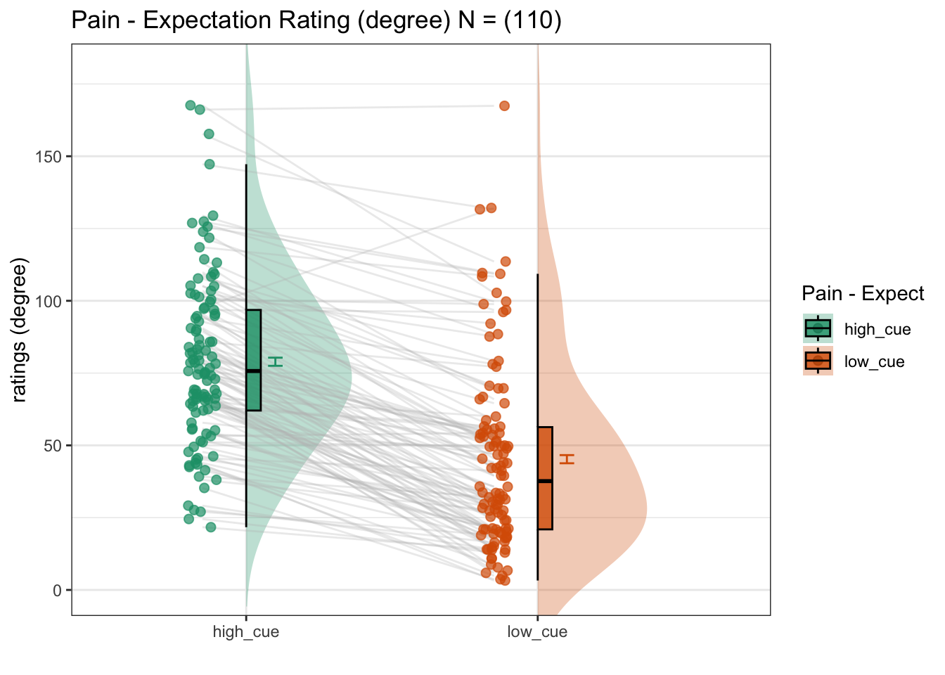
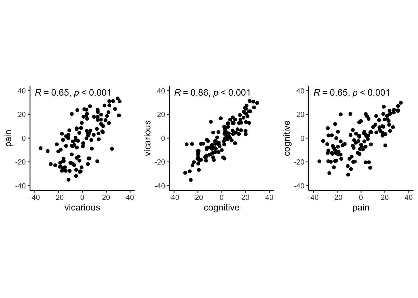
2.4 Individual difference analysis
Are cue effects (on expectation ratings) similar across tasks?
Using the random slopes of cue effects, here we plot them side by side with all three tasks of pain, cognitive, vicarious. As we can see, there is a high correlation across the random effects of cue across pain-cognitive, pain-vicarious, and cognitive-vicarious. These plots suggest a universal mechansim in the cue-expectancy effect, although some may critic that the cues were identical across tasks, thereby the cue effects are identical due to the stimuli itself, not necessarily a domain-general expectation process.
## Warning: Removed 3 rows containing non-finite values (`stat_cor()`).## Warning: Removed 3 rows containing missing values (`geom_point()`).## Warning: Removed 1 rows containing non-finite values (`stat_cor()`).## Warning: Removed 1 rows containing missing values (`geom_point()`).## Warning: Removed 3 rows containing non-finite values (`stat_cor()`).## Warning: Removed 3 rows containing missing values (`geom_point()`).