9 beh :: Different scaling methods ~ Cue effects
What is the purpose of this notebook?
Here, we extract the cue effects across different types of ratings * cue effects of raw outcome rating (“cue_raw_outcome”) * cue effects of z-scored outcome rating (“cue_z_outcome”) * stim effects of raw outcome rating (“stim_raw_outcome”) * stim effects of z-scored outcome rating (“stim_z_outcome”) * cue effects / stim effect using raw outcome rating (“cuestim_raw_outcome”) * cue effects / stim effects using z score ratings (“cuestim_z_outcome”) * regularized cue effects +1 / stim effect +1 using raw outcome rating (“cuestim_raw_outcome_reg”) * regularized cue effects / stim effects using z score ratings (“cuestim_z_outcome_reg”)
load libraries
library(car)
library(psych)
library(lme4); library(lmerTest)
library(glmmTMB)
library(plyr)
library(dplyr)
library(cueR)
library(ggplot2)
library(plotly)
library(gridExtra)
library(broom.mixed)
library(knitr)
library(grid)
library(ggpubr)

library(dplyr)
library(broom.mixed)
library(effectsize)
library(corrplot)
compute_enderstofighi <- function(data, sub, outcome, expect, ses, run) {
  maindata <- data %>%
    group_by(!!sym(sub)) %>%
    mutate(OUTCOME = as.numeric(!!sym(outcome))) %>%
    mutate(EXPECT = as.numeric(!!sym(expect))) %>%
    mutate(OUTCOME_cm = mean(OUTCOME, na.rm = TRUE)) %>%
    mutate(OUTCOME_demean = OUTCOME - OUTCOME_cm) %>%
    mutate(EXPECT_cm = mean(EXPECT, na.rm = TRUE)) %>%
    mutate(EXPECT_demean = EXPECT - EXPECT_cm) %>%
    #mutate(OUTCOME_zscore = as.numeric(scale(OUTCOME, center = TRUE, scale = TRUE)[, 1])) %>%
    #mutate(EXPECT_zscore = as.numeric(scale(EXPECT, center = TRUE, scale = TRUE)[, 1]))
    mutate(OUTCOME_zscore = (OUTCOME - mean(OUTCOME, na.rm = TRUE))/sd(OUTCOME, na.rm = TRUE)) %>% #as.numeric(scale(OUTCOME, center = TRUE, scale = TRUE)[, 1])) %>%
    mutate(EXPECT_zscore = (EXPECT - mean(EXPECT, na.rm = TRUE))/sd(EXPECT, na.rm = TRUE)) #as.numeric(scale(EXPECT, center = TRUE, scale = TRUE)[, 1]))

  data_p2 <- maindata %>%
    arrange(!!sym(sub)) %>%
    group_by(!!sym(sub)) %>%
    mutate(trial_index = row_number())

  data_a3 <- data_p2 %>%
    group_by(!!sym(sub), !!sym(ses), !!sym(run)) %>%
    mutate(trial_index = row_number(!!sym(run)))

  data_a3lag <- data_a3 %>%
    group_by(!!sym(sub), !!sym(ses), !!sym(run)) %>%
    mutate(lag.OUTCOME_demean = dplyr::lag(OUTCOME_demean, n = 1, default = NA))

  # Create Subjectwise Mean, centered in relation to the group mean
  data_a3cmc <- data_a3lag %>%
    ungroup %>%
    mutate(EXPECT_cmc = EXPECT_cm - mean(EXPECT_cm, na.rm=TRUE)) %>%
    mutate(OUTCOME_cmc = OUTCOME_cm - mean(OUTCOME_cm, na.rm=TRUE))


  # Remove NA values ___________________________________________________________
  data_centered_NA <- data_a3cmc %>%
    filter(!is.na(OUTCOME)) %>% # Remove NA values
    filter(!is.na(EXPECT))

  return(data_centered_NA)

}
9.0.1 display distribution of data
Let’s look at the distribution of the data. X axis: Y axis:
head(df.PVC_center)## # A tibble: 6 × 33
## src_subject_id session_id param_run_num param_task_name event02_expect_angle
## <int> <int> <int> <chr> <dbl>
## 1 2 1 1 pain 5.53
## 2 2 1 1 pain 18.9
## 3 2 1 1 pain 103.
## 4 2 1 1 pain 81.2
## 5 2 1 1 pain 97.2
## 6 2 1 1 pain 117.
## # ℹ 28 more variables: param_cue_type <chr>, param_stimulus_type <chr>,
## # event04_actual_angle <dbl>, trial_index <int>, trial_count_sub <int>,
## # trial_ind <dbl>, sub <chr>, ses <chr>, run <chr>, runtype <chr>,
## # task <chr>, trial_sub <int>, trial <chr>, cuetype <chr>,
## # stimintensity <chr>, DEPc <chr>, DEP <chr>, OUTCOME <dbl>, EXPECT <dbl>,
## # OUTCOME_cm <dbl>, OUTCOME_demean <dbl>, EXPECT_cm <dbl>,
## # EXPECT_demean <dbl>, OUTCOME_zscore <dbl>, EXPECT_zscore <dbl>, …
#colnames(df.PVC_center)Summary:
9.1 function: compute cue effects
#' Compute Cue Effect
#'
#' This function processes a dataframe to compute the cue effect. It involves
#' subsetting and filtering the data, summarizing conditions, calculating
#' difference scores, and calculating group-wise contrast. The function also
#' allows renaming of the resultant columns.
#'
#' @param df A dataframe containing the relevant data.
#' @param dv The name of the dependent variable in the dataframe.
#' @param new_col_name The new name for the column that will be created as a result
#'        of computing the cue effect.
#' @return A dataframe with the computed cue effect, sorted by task, with a new
#'         column for the cue effect and its standard deviation, renamed as specified.
#' @import dplyr
#' @import tidyr
#' @import Rmisc
#' @export
#' @examples
#' # Assuming df is a dataframe with the necessary structure and "OUTCOME" is your dependent variable:
#' result <- compute_cueeffect(df, "OUTCOME", "new_cue_effect")
compute_cueeffect <- function(df, dv, new_col_name) {
  library(dplyr)
  library(tidyr)
  library(Rmisc)

  # 1) Subset and filter data __________________________________________________
  df$task <- factor(df$task)
  sub_diff <- subset(df, select = c("sub", "ses", "run", "task", "stimintensity", "cuetype", dv))
  sub_diff_NA <- sub_diff %>% filter(!is.na(dv))

  # 2) Summarize each condition and spread out columns _________________________
  subjectwise <- meanSummary(sub_diff_NA, c("sub", "ses", "run", "task", "cuetype", "stimintensity"), dv)
  mean_outcome <- subjectwise[1:(length(subjectwise) - 1)]
  wide <- mean_outcome %>% tidyr::spread(cuetype, mean_per_sub)

  # 3) Calculate difference score ______________________________________________
  wide$diff <- wide$`cuetype-high` - wide$`cuetype-low`
  subjectwise_diff <- meanSummary(wide, c("sub", "task"), "diff")
  subjectwise_NA <- subjectwise_diff %>% filter(!is.na(sd))

  # 4) Calculate group wise contrast ___________________________________________
  groupwise_diff <- summarySEwithin(data = subjectwise_NA, measurevar = "mean_per_sub", withinvars = "task", idvar = "sub")
  sd_col <- paste0(new_col_name, "_sd")
  # sort data based on task and rename _________________________________________
  sorted_df <- subjectwise_diff %>%
    arrange(task) %>%
    rename(!!new_col_name := mean_per_sub,
           !!sd_col := sd
           )

  return(sorted_df)
}
9.2 function: compute stim effects
#' Compute Stimulus Effect
#'
#' This function calculates the stimulus effect based on the provided dataframe.
#' It filters the data, computes summary statistics, calculates difference scores,
#' and optionally renames the resulting columns.
#'
#' @param df Dataframe containing the data to be analyzed.
#' @param dv Name of the dependent variable column in `df`.
#' @param new_col_name New column name for the renamed mean_per_sub column.
#' @return A dataframe with the computed stimulus effect, sorted by task,
#'         and with columns optionally renamed.
#' @import dplyr
#' @import tidyr
#' @import Rmisc
#' @export
#' @examples
#' # Assuming df is your dataframe and "OUTCOME" is your dependent variable:
#' result <- compute_stimeffect(df, "OUTCOME", "new_mean_outcome")
compute_stimeffect <- function(df, dv, new_col_name) {
  # 1) Subset and filter data __________________________________________________
  df$task <- factor(df$task)
  sub_diff <- subset(df, select = c("sub", "ses", "run", "task", "stimintensity", "cuetype", dv))
  sub_diff_NA <- sub_diff %>% filter(!is.na(dv))


  # 2) Summarize each condition and spread out columns _________________________
  subjectwise <- meanSummary(sub_diff_NA, c("sub", "ses", "run", "task", "cuetype", "stimintensity"), dv)
  mean_outcome <- subjectwise[1:(length(subjectwise) - 1)]
  wide <- mean_outcome %>% tidyr::spread(stimintensity, mean_per_sub)

  # 3) Calculate difference score ______________________________________________
  wide$diff <- wide$high - wide$low
  subjectwise_diff <- meanSummary(wide, c("sub", "task"), "diff")
  subjectwise_NA <- subjectwise_diff %>% filter(!is.na(sd))
  #
  # # 4) Calculate group wise contrast _________________________________________
  groupwise_diff <- Rmisc::summarySEwithin(data = subjectwise_NA,
                                           measurevar = "mean_per_sub",
                                           withinvars = "task",
                                           idvar = "sub")
  #
  sd_col <- paste0(new_col_name, "_sd")
  # sort data based on task and rename _________________________________________
  sorted_df <- subjectwise_diff %>%
    arrange(task) %>%
    rename(!!new_col_name := mean_per_sub,
           !!sd_col := sd
           )
  return(sorted_df)
}
compute the cue and stim effects for further analysis
# calculate cue & stim effects per participant and rename column _______________
cue_raw_outcome <- compute_cueeffect(df.PVC_center, dv = "OUTCOME", new_col_name = "cue_raw_outcome")
##
## Attaching package: 'tidyr'## The following objects are masked from 'package:Matrix':
##
## expand, pack, unpack## Loading required package: lattice##
## Attaching package: 'Rmisc'## The following objects are masked from 'package:cueR':
##
## normDataWithin, summarySE
cue_z_outcome <- compute_cueeffect(df.PVC_center, dv = "OUTCOME_zscore", new_col_name = "cue_z_outcome")
cue_raw_expect <- compute_cueeffect(df.PVC_center, dv = "EXPECT", new_col_name = "cue_raw_expect")
cue_z_expect <- compute_cueeffect(df.PVC_center, dv = "EXPECT_zscore", new_col_name = "cue_z_expect")

rawstim_outcome <- compute_stimeffect(df.PVC_center, dv = "OUTCOME", new_col_name = "stim_raw_outcome")
zstim_outcome <- compute_stimeffect(df.PVC_center, dv = "OUTCOME_zscore", new_col_name = "stim_z_outcome")
rawstim_expect <- compute_stimeffect(df.PVC_center, dv = "EXPECT", new_col_name = "stim_raw_expect")
zstim_expect <- compute_stimeffect(df.PVC_center, dv = "EXPECT_zscore", new_col_name = "stim_z_expect")


# Merging all dataframes _______________________________________________________
merged_df <- cue_raw_outcome %>%
  full_join(cue_z_outcome, by = c("sub", "task")) %>%
  full_join(cue_raw_expect, by = c("sub", "task")) %>%
  full_join(cue_z_expect, by = c("sub", "task")) %>%
  full_join(rawstim_outcome, by = c("sub", "task")) %>%
  full_join(zstim_outcome, by = c("sub", "task")) %>%
  full_join(rawstim_expect, by = c("sub", "task")) %>%
  full_join(zstim_expect, by = c("sub", "task"))

# calculate cue vs stim effect ratio ___________________________________________
merged_df$cuestim_raw_outcome <- merged_df$cue_raw_outcome/merged_df$stim_raw_outcome
merged_df$cuestim_raw_outcome_reg <- (merged_df$cue_raw_outcome+1)/(merged_df$stim_raw_outcome+1)

merged_df$cuestim_z_outcome <- merged_df$cue_z_outcome/merged_df$stim_z_outcome
merged_df$cuestim_z_outcome_reg <- (merged_df$cue_z_outcome+1)/(merged_df$stim_z_outcome+1)


write.csv(merged_df, file.path(main_dir, "data", "hlm", "cue_stim_effects_scaling.csv"), row.names = FALSE)
# Let's check what the cue & stim effects look like ____________________________
head(merged_df)
## sub task cue_raw_outcome cue_raw_outcome_sd cue_z_outcome
## 1 sub-0002 cognitive 4.540887 6.343282 0.12174487
## 2 sub-0003 cognitive 7.636581 17.103371 0.47159597
## 3 sub-0004 cognitive 1.627529 7.632712 0.07069328
## 4 sub-0005 cognitive 13.130997 41.442596 0.33303376
## 5 sub-0006 cognitive 5.148439 28.946650 0.15567303
## 6 sub-0007 cognitive 14.076683 9.627143 0.63495614
## cue_z_outcome_sd cue_raw_expect cue_raw_expect_sd cue_z_expect
## 1 0.1700686 23.90350 18.73398 0.5963963
## 2 1.0562162 30.15502 25.17697 1.2605728
## 3 0.3315341 33.77405 25.34289 1.0873435
## 4 1.0510842 41.78567 37.36012 1.2517185
## 5 0.8752581 30.56264 19.98909 1.0611074
## 6 0.4342510 29.32456 11.57591 1.1869398
## cue_z_expect_sd stim_raw_outcome stim_raw_outcome_sd stim_z_outcome
## 1 0.4674160 4.4896815 10.040412 0.12037201
## 2 1.0524748 4.0612018 11.029078 0.25079893
## 3 0.8159054 0.9329999 6.238765 0.04052574
## 4 1.1191483 4.6718609 29.829606 0.11848966
## 5 0.6940032 15.8650585 28.858031 0.47971082
## 6 0.4685462 12.5187276 11.450963 0.56468155
## stim_z_outcome_sd stim_raw_expect stim_raw_expect_sd stim_z_expect
## 1 0.2691916 -3.343426 20.107224 -0.08341906
## 2 0.6810991 -4.285159 7.409842 -0.17913285
## 3 0.2709867 -1.031139 9.824031 -0.03319716
## 4 0.7565508 -2.959005 8.839276 -0.08863904
## 5 0.8725786 7.058330 18.466885 0.24505886
## 6 0.5165180 -4.460202 9.261081 -0.18053095
## stim_z_expect_sd cuestim_raw_outcome cuestim_raw_outcome_reg
## 1 0.5016787 1.0114051 1.0093276
## 2 0.3097542 1.8803747 1.7064289
## 3 0.3162812 1.7444044 1.3593012
## 4 0.2647866 2.8106567 2.4914216
## 5 0.6411536 0.3245143 0.3645667
## 6 0.3748512 1.1244500 1.1152442
## cuestim_z_outcome cuestim_z_outcome_reg
## 1 1.0114051 1.0012254
## 2 1.8803747 1.1765248
## 3 1.7444044 1.0289926
## 4 2.8106567 1.1918159
## 5 0.3245143 0.7810128
## 6 1.1244500 1.0449130
pain.df <-merged_df[merged_df$task == 'pain', ]
cor(pain.df$cue_raw_outcome, pain.df$cue_z_outcome, use = "complete.obs")
## [1] 0.9155303
# Reshape the dataframe to a long format _______________________________________
pain.long_df <- pivot_longer(pain.df,
                        cols = c("cue_raw_outcome", "cue_z_outcome",
                                 "cue_raw_expect", "cue_z_expect",
                                 "stim_raw_outcome", "stim_z_outcome",
                                 "stim_raw_expect", "stim_z_expect",

                                 "cuestim_raw_outcome", "cuestim_raw_outcome_reg",
                                 "cuestim_z_outcome", "cuestim_z_outcome_reg"
                                 ),
                        names_to = "variable",
                        values_to = "value")

pain_heatmap <- pain.long_df[, c("sub", "variable", "value")]
# Create the heatmap ___________________________________________________________
ggplotly(ggplot(pain_heatmap, aes(x = variable, y = sub, fill = value)) +
  geom_tile() +
  scale_fill_gradient(low = "blue", high = "red") +
  #facet_grid(rows = vars(sub)) +
  theme_minimal() +
  coord_fixed(ratio = .1) +
  labs(x = "Variable", y = "Subject", fill = "Value") +
   theme(axis.text.x = element_text(angle = 45, hjust = 1),
        axis.text.y = element_text(angle = 45, vjust = 1)))
# correlation matrix ___________________________________________________________
pain.df.subset <- pain.df[, c("cue_raw_outcome", "cue_z_outcome",
"cue_raw_expect", "cue_z_expect",
"stim_raw_outcome", "stim_z_outcome",
"stim_raw_expect", "stim_z_expect",
"cuestim_raw_outcome", "cuestim_raw_outcome_reg",
"cuestim_z_outcome", "cuestim_z_outcome_reg")]
#"cuestim_raw_expect", "cuestim_raw_expect_reg",
#"cuestim_z_expect", "cuestim_z_expect_reg")]
M <- cor(as.matrix(pain.df.subset), use ="complete.obs")
#round(M, 2)
testRes = cor.mtest(M, conf.level = 0.95)
corrplot(M, p.mat = testRes$p, method = 'color', diag = TRUE,
sig.level = c( 0.05), pch.cex = 0.7,
tl.cex = 0.6,
insig = 'label_sig', pch.col = 'grey20')#, order = 'AOE')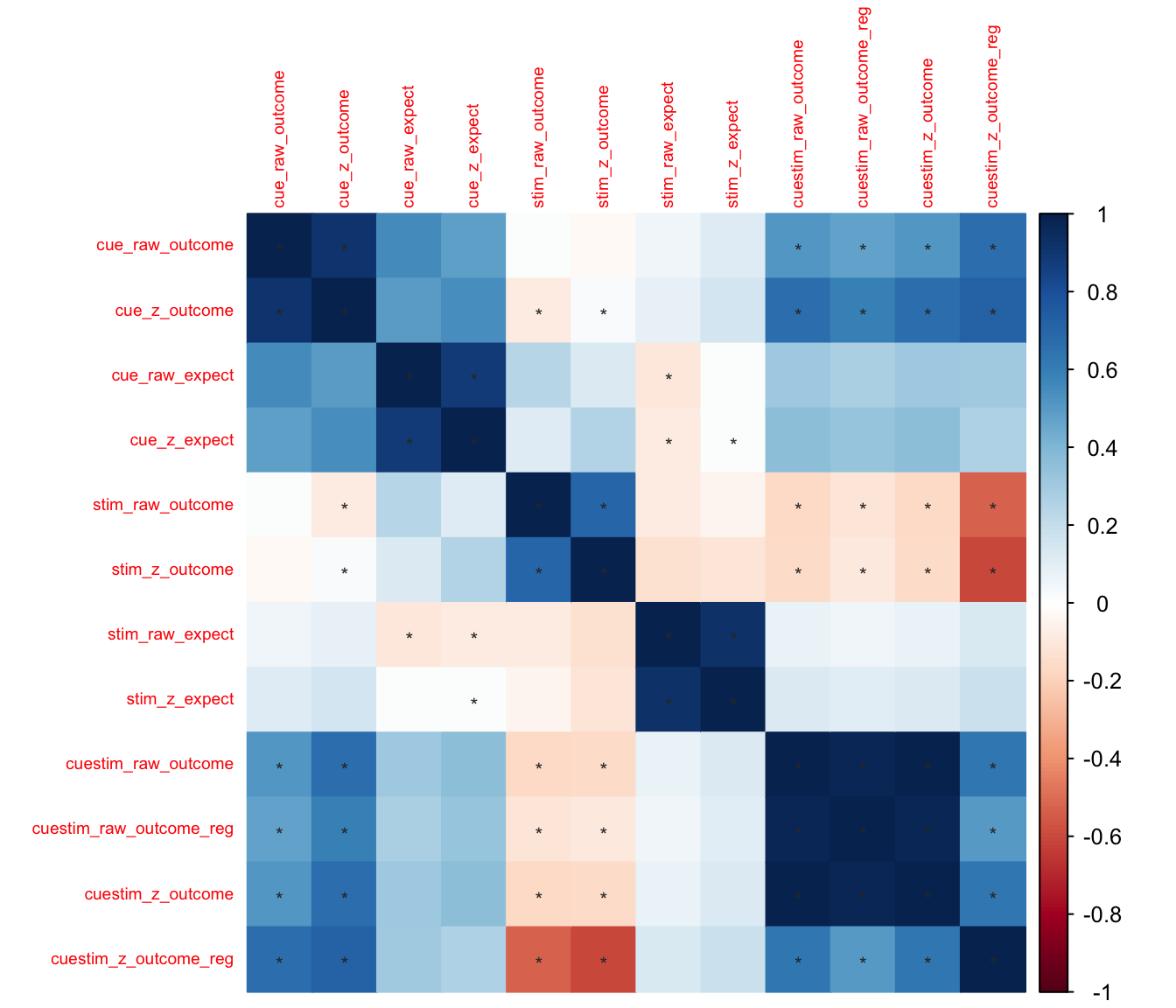 ## Illustration of the plot labels
The variable names indicate
## Illustration of the plot labels
The variable names indicate {effect}_{raw/z}_{ratings}
-
effectillustrates which contrasts we compute, cue effects or stim effects-
cue: high cue vs. low cue average values per participant -
stim: high stim vs. low stim average values per participant
-
-
raw/z:-
raw: use the raw behavioral ratings (per participant) to compute the aforementioned effects, or -
z: use the z scores (per participant) to compute the aforementioned effects
-
-
ratings-
outcome: outcome ratings -
expect: expectation ratings
-
- example:
cue_raw_outcomeillustrate the cue effect, calculated based on raw outcome ratings. It is the average outcome rating difference between high vs. low cues, calculated per participant.
9.3 Summary:
- Given that these cue-effect scores are between subject measures, the Z scored version and the raw scored version will have the same variance structure across participants.
- Taking a look at the correlation matrix,
- we know what raw and z scores of the same effects will have a significant correlation.
- Validation:
- expectation ratings as a function of cue (“cue_raw_expect”) are highly correlated with outcome ratings as a function of cue (“cue_raw_outcome”).
- Stimulus effects have no correlation with the cue effects (i.e. there is no significant corerlation of “stim_raw_outcome” & “cue_raw_outcome” ).
- Question: cue effect proportional to the stim effect (“cuestim_raw_outcome”) is correlated with the stim effect, but not the cue effect. why?
rand_norms_100 <- rnorm(n = 100, mean = 100, sd = 25)
rand_norms_100.Z <- (rand_norms_100-mean(rand_norms_100))/sd(rand_norms_100)
cor(rand_norms_100, rand_norms_100.Z)
## [1] 1
rand_norms_100.demean <- (rand_norms_100-mean(rand_norms_100))
cor(rand_norms_100, rand_norms_100.demean)
## [1] 1